User Manual#
Introduction#
This manual aims to guide the end users in the application of InVesalius tools. The manual also presents some concepts to facilitate the use of the software.
Important Concepts#
Detailed in this section is a list of concepts essential to better understand and operate the software.
DICOM (Digital Image Communications in Medicine)#
DICOM is a standard the transmission, storage and treatment of medical images. The standard encompasses various origins of medical images, such as images emanating from computed tomography (CT) equipment, magnetic resonance, ultrasound, and electrocardiogram, among others.
A DICOM image consists of two main components, namely, an array containing the pixels of the image and a set of meta-information. This information includes, but is not limited to, patient name, mode image and the image position in relation to the space (in the case of CT and MRI).
Computed Tomography — Medical#
Computed tomography indicates the radiodensity of tissues, i.e., the average X-ray absorption by the tissues. The radiodensity reading is translated into an image gray levels, called the Hounsfield scale, named Godfrey Newbold Hounsfield, one of the creators of the first CT scan.
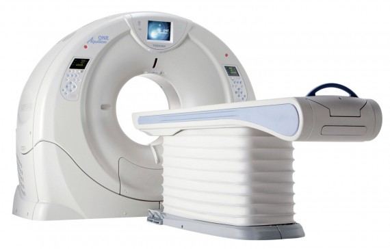
Fig. 1 Meidcal CT scanner - www.toshibamedical.com.br#
Most modern CT scanning appliances are equipped with a radiation emitter and a sensor bank (with channels ranging from 2 to 256), which circle the patient while the stretcher is moved, forming a spiral. This generates a large number of images simultaneously, with little emission of X-rays.
Hounsfield Scale#
As mentioned in the previous section, the CT images are generated in gray levels, expressed in Hounsfield (HU), wherein lighter shades represent denser matter, and the darker, less dense matter such as skin and brain tissue.
The table below presents some materials and their respective values in Hounsfield Units (HU).
Material |
HU |
|---|---|
Air |
-1000 or less |
Fat |
-120 |
Water |
0 |
Muscle |
40 |
Contrast |
130 |
Bone |
400 or more |
Computed Tomography - Dental (CBCT)#
Dental CT commonly works with less radiation emission compared to medical CT, and therefore makes it possible to view more details of delicate regions such as alveolar cortical.
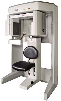
Fig. 2 Dental tomography - www.kavo.com.br#
Image acquisition is performed with the patient positioned vertically (as opposed to medical tomography in which the patient is horizontal). A transmitter X-ray surrounds the patient’s skull, forming an arc of 180° or 360°. The images generated are compiled as a volume of the patient’s skull. This volume is then “sliced” by the software into individual layers, being able to generate images with different spacing or fields of view, such as a panoramic view of the region of interest.
The images acquired by dental scanners often require more post-processing when it is necessary to separate (segmental) certain structures using other software such as InVesalius. This is because, typically, these images have more gray levels than, which makes use of segmentation patterns (preset) less. Another very common feature in the images of provincial dental CT scanners is the high presence of speckle noise and other forms of noise typically caused by the presence of amalgam prosthetics.
Magnetic Resonance Imaging - MRI#
MRI is an examination performed without the use of ionizing radiation. Instead, it uses a strong magnetic field to align the atoms of any element present in our body, most commonly hydrogen. After alignment, radio waves are triggered to excite atoms. The sensors measure the time that the hydrogen atoms take to realign. This makes it possible to distinguish between different tissues, as different types possess different quantities of hydrogen atoms.
To avoid interference and improve the quality of the radio frequency signal, the patient is placed inside a narrow tube encompassed by the coil and scanning unit.
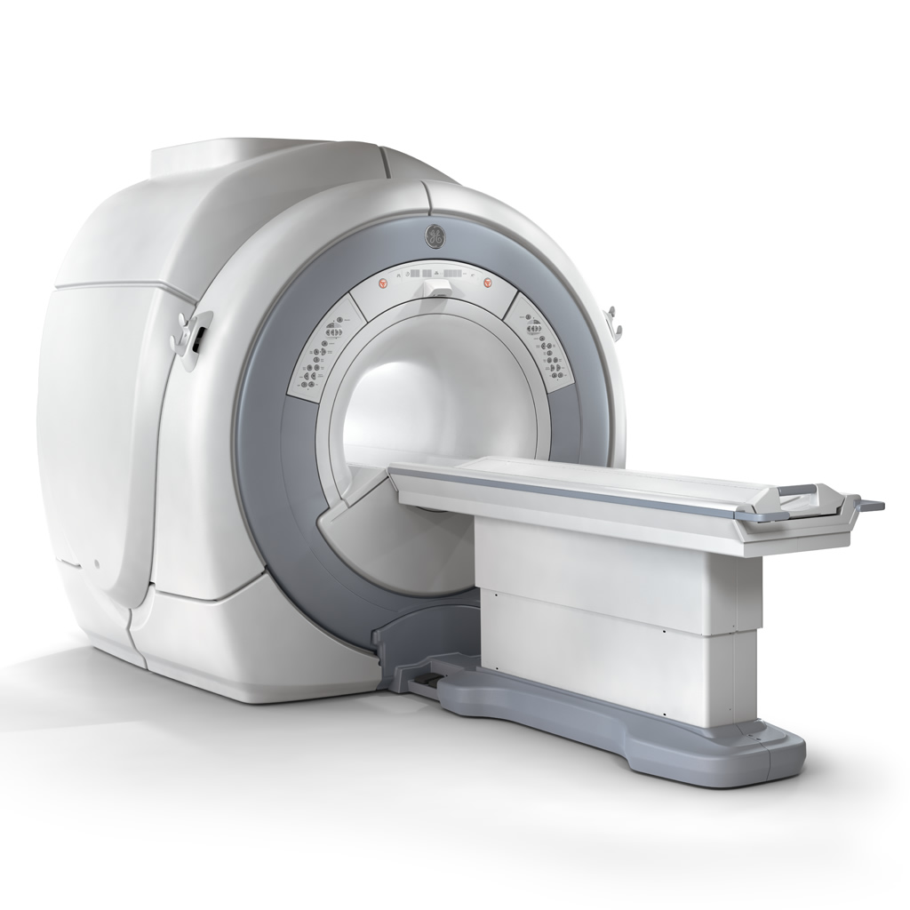
Fig. 3 Magnetic resonance imaging equipment - www.gehealthcare.com#
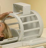
Fig. 4 Coil - www.healthcare.philips.com#
Software and Hardware Requirements#
InVesalius is designed to run on personal computers, such as desktops and notebooks. Currently, it is compatible with the following operating systems:
Microsoft Windows (Windows 7, 8, 10)
GNU/Linux (Ubuntu, Mandriva, Fedora)
Apple macOS
However, Windows offers the most stable performance and the easiest setup.
The performance of InVesalius depends mainly on the number of
reconstructed slices (images offered by the software), the amount of
random access memory (RAM) available, the processor clock rate &
frequency, and operating system architecture (32-bit or 64-bit).
It is important to note that, as a general rule, the greater the amount of RAM available on the system, the larger the number of slices that can be opened simultaneously. For example, with 1 GB of available memory, it can open about 300 slices with a resolution of 512x512 pixels. With 4 GB of memory, around 1000 images can be opened simultaneously at the same resolution.
Minimum Computer Settings#
32-bit Operating System
Intel Pentium 4 or equivalent 1.5 GHz
1 GB of RAM
10 GB available hard disk space
Graphics card with 64 MB memory
Video resolution of 1024x768 pixels
Recommended Computer Settings#
64-bit Operating System
Intel i7 or equivalent processor
16 GB of RAM
20 GB available hard disk space
Geforce or AMD or Quadro (P2000 equivalent or superior) graphics card
Video resolution of 1920x1080 pixels
Installation#
To download InVesalius, visit one of the following sites:
MS-Windows#
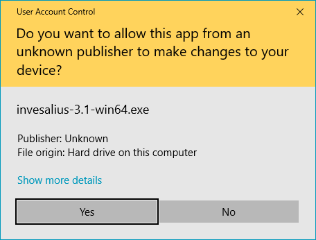
To install InVesalius on MS-Windows, simply run the installer program. When a window asking you to confirm the file execution appears, click Yes.
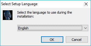
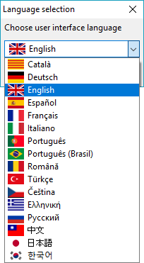
A new window will ask you to select the language of the installer. Select the language and click OK.
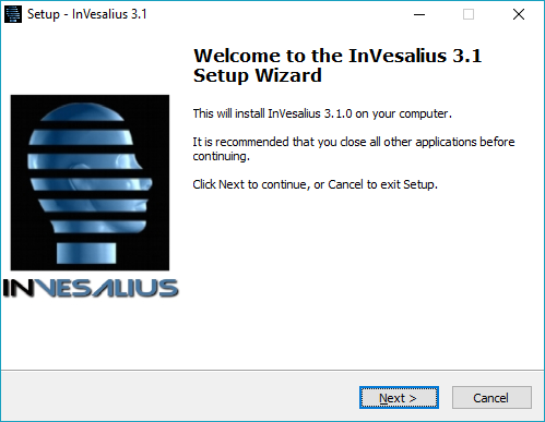
The Setup installer will appear. Click Next.
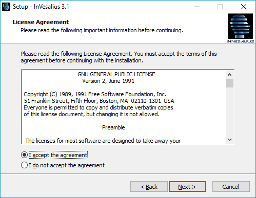
Select I accept the agreement and click the Next button.
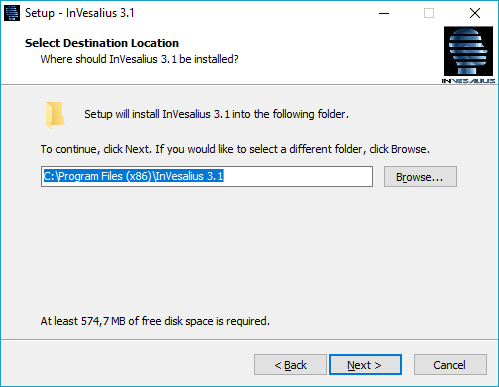
Select the preferred destination for the InVesalius program files, then click Next.
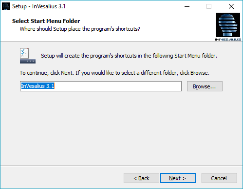
Click the Next button.
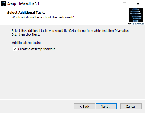
Select Create a desktop shortcut and click Next.
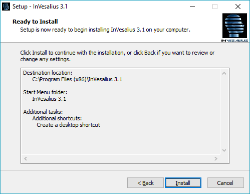
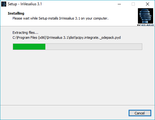
Click the Install button.
While the software is being installed, a progress window will appear.
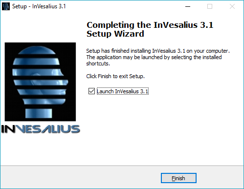
To run InVesalius after installation, check Launch InVesalius 3.1 and click the Finish button.
When being run for the first time, a window will appear to select the InVesalius language. Select the desired language and click OK.
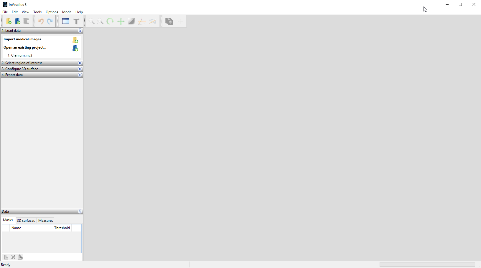
While InVesalius is loading, the opening window shown below will be displayed.
The main program window will then open, as shown below.
MacOS#
To start the installation on macOS, double-click the installer with the left mouse button to begin installation.
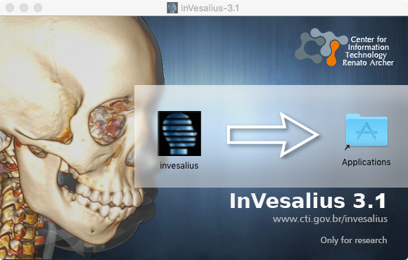
Hold down the left button on the InVesalius software icon and drag it to the Applications folder. Both are contained in the installer.
The software is now installed and can be accessed through the menu.
Image Import#
InVesalius imports files in DICOM format, including compressed files (lossless JPEG), Analyze (Mayo Clinic©), NIfTI, PAR/REC, BMP, TIFF, JPEG and PNG formats.
DICOM#
Under the File menu, click on Import DICOM or use the shortcut Ctrl+I. Additionally, DICOM files can be imported by clicking on the icon shown in Fig. 5.

Fig. 5 Shortcut to DICOM import#
Select the directory containing the DICOM files, as in Fig. 6. InVesalius will search for files also in subdirectories of the chosen directory if they exist.
Once the directory is selected, click OK.
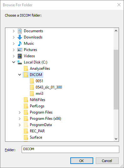
Fig. 6 Folder selection#
While InVesalius search for DICOM files in the directory, the loading progress of the scanned files is displayed, as shown in the Fig. 7.
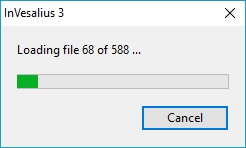
Fig. 7 Loading file status#
If DICOM files are found, a window open (shown Fig. 8) will open to select the patient and respective series to be opened. It is also possible to skip images for reconstruction.
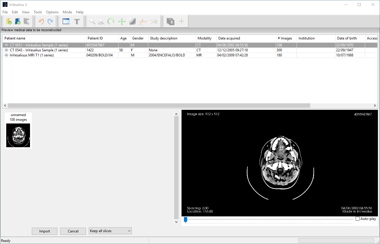
Fig. 8 Import window#
To import a series with all images present, click “+”\ on the patient’s name to expand the corresponding series. Double-click on the description of the series. See Fig. 9.
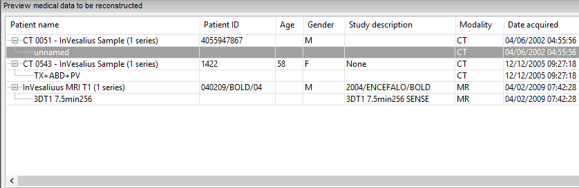
Fig. 9 Series selection#
In some cases, when there is no computer with memory and/or satisfactory processing to work with large numbers of images in a series, it is recommended to skip some of them. To do this, click once with the left mouse button over the description of the series (Fig. 9) and select how many images will be skipped (Fig. 10), then click Import.
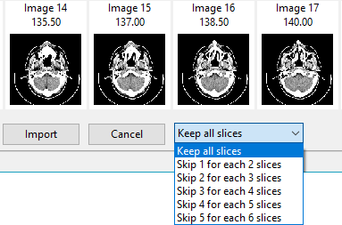
Fig. 10 Skip image option#
If there is an insufficient amount of available memory at the time of loading the images, it is recommended that the resolution of the slices be reduced to work with volumetric and surface visualization, as shown in Fig. 11. The slices will be resized according to the percentage relative to the original resolution. For example, if each slice of the exam the dimension of 512 x 512 pixels and the “Percentage of original resolution” is suggested to be 60 %, each resulting image will be 307 x 307 pixels. To open with the original pixel resolution, set the percentage to 100.
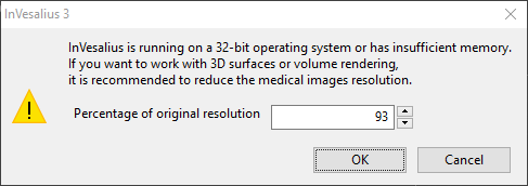
Fig. 11 Image size reduction#
If the image was obtained with the gantry tilted, it will be necessary to correct to avoid distortion of any reconstruction. InVesalius allows the user to do this easily. When importing an image with the gantry tilted a dialog will appear, showing the gantry tilt angle. (Fig. 12). It is possible to change this value, but it is not recommended. Click on the Ok to do the correction. If you click on the Cancel button, the correction will not be done.
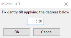
Fig. 12 Gantry tilt correction#
After the above procedure, a window will be displayed (Fig. 13) with reconstruction (when images are stacked and interpolated).
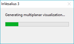
Fig. 13 Reconstruction progress#
Analyze#
To import Analyze files, under the File menu, click Import other files, then click on the Analyze option as show the Fig. 14.
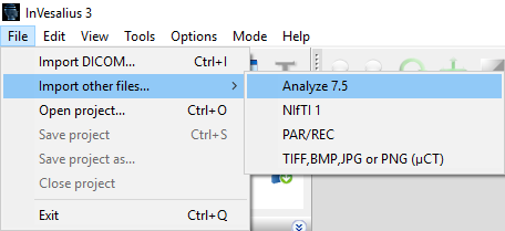
Fig. 14 Menu for importing images in analyze format.#
Select the Analyze file format (.hdr) and click on Open (Fig. 15).
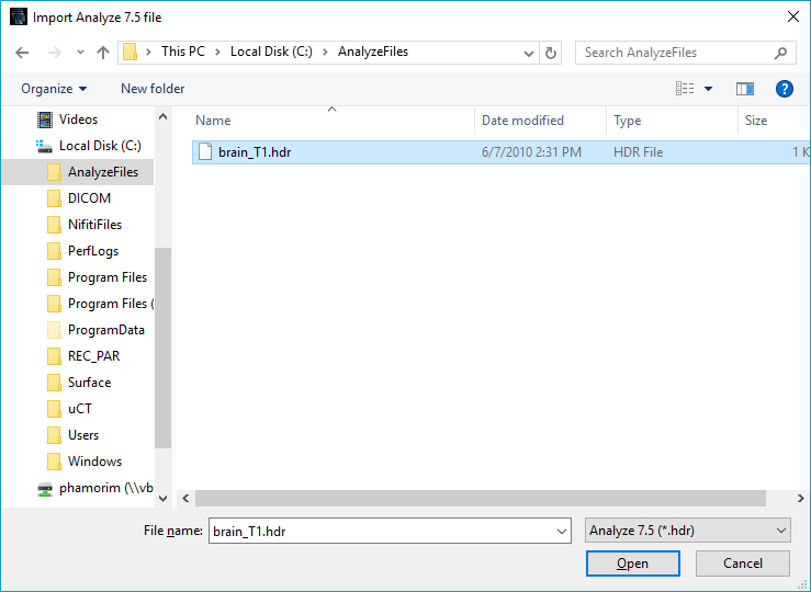
Fig. 15 Import analyze file format.#
NIfTI#
To import NIfTI files, under the File menu, click Import other files and then click NIfTI as shown in Fig. 16.
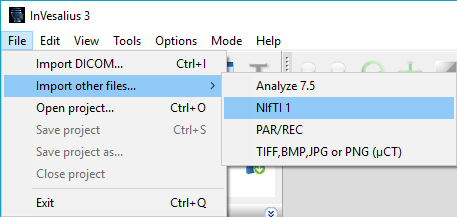
Fig. 16 Menu to import images in NIfTI format#
Select the NIfTI file format (either nii.gz or .nii) then click Open (Fig. 17). If the file is in another format as .hdr, select all files(*.*) option.
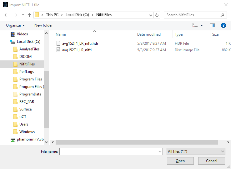
Fig. 17 Importing images in NIfTI format.#
PAR/REC#
To import PAR/REC file, under the File menu, click Import other files, and then click on PAR/REC as shown in Fig. 18.

Fig. 18 Menu for importing PAR/REC images#
Select PAR/REC file type with the file extension .par and click Open (Fig. 19). If the file has no extension, select all files(*.*) option.
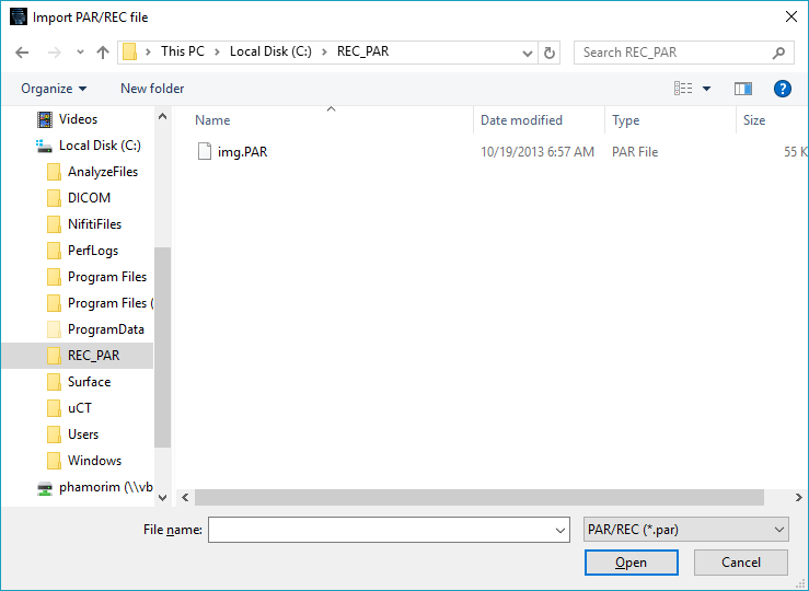
Fig. 19 PAR/REC import#
TIFF, JPG, BMP, JPEG or PNG (micro-CT)#
TIFF, JPG, BMP, JPEG or PNG file format for microtomography equipment (micro-CT or µCT) or others. InVesalius imports files in these formats if pixels present are represented in grayscale.
To import, click on menu File, Import other files… and then click on TIFF, JPG, BMP, JPEG or PNG (µCT) option as shown in the Fig. 20.
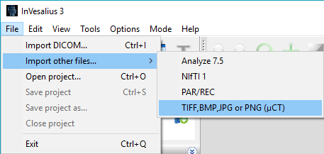
Fig. 20 Import images in BMP and others formats#
Select the directory that contains the files, as shown the Fig. 21. InVesalius will search for files also in subdirectories of the chosen directory if they exist.
Click on OK.
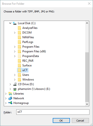
Fig. 21 Folder selection#
While InVesalius is looking for TIFF, JPG, BMP, JPEG, or PNG files in the directory, the upload progress of the scanned files is displayed, as illustrated in Fig. 22.
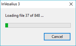
Fig. 22 Checking and loading files status.#
If files in the desired formats are located, a window will open (shown in Fig. 23) to display the files eligible for reconstruction. Images can also be skipped to remove files from the rebuild list. The files are sorted according to file names. It is recommended that the files are numbered according to the desired rebuild order.
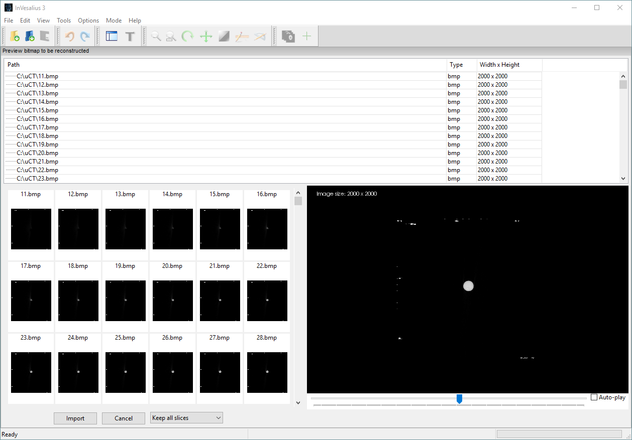
Fig. 23 Window to import BMP files.#
To delete files that are not of interest, select a file by clicking the left mouse button and then pressing the delete key. You can also choose a range of files to delete by clicking the left mouse button on a file, holding down the shift key, clicking again with the mouse button in the last file of the track and finally pressing the delete button.
Similar to when importing DICOM files, you can skip BMP images for re-building. In some cases, particularly where a computer with satisfactory memory and/or processing is unavailable, it may be advisable to skip some of them to retain adequate program functionality. To do this, select how many images to skip (Fig. 24), then click Import.
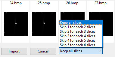
Fig. 24 Importation window#
To reconstruct files of this type, a project name must be defined to indicate the orientation of the images (axial, coronal or sagittal), voxel spacing (X, Y and Z) in mm as shown in the Fig. 25. The voxel spacing in X is the pixel width of each image, Y the pixel length, and Z represents the distance of each slice (voxel height).
If the image set consists of microtomography images, more specifically GE and Brucker equipment, it is possible that InVesalius will read the text file with the acquisition parameters that normally stay in the same folder as the images and automatically insert the spacing. This verification can be done when the values of X, Y and Z are different from “1.00000000”, otherwise it is necessary to enter the values of the respective spacing.
Correct spacing is crucial for correctly importing objects in InVesalius. Incorrect spacing will provide incorrect measurements.
Once all parameters have been input, click OK.
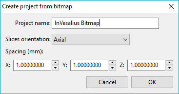
Fig. 25 Import screen#
If insufficient memory is available when loading images, it is recommended to reduce the resolution of the slices to work with volumetric and surface visualization, as shown in Fig. 26 window.The slices will be resized according to the percentage relative to the original resolution. For example, if each slice of the exam contains the dimension of 512 x 512 pixels and the “Percentage of the original resolution” is suggested at 60, each resulting image will have 307 x 307 pixels. If you want to open with the original resolution, set the percentage to 100.
Fig. 26 Image resize#
After the previous steps, wait a moment for the program to complete the multiplanar reconstruction as shown in Fig. 27.
Fig. 27 Multiplanar reconstruction in progress.#
Image Adjustment#
InVesalius cannot guarantee the correct image order; images may contain incorrect information, or do not follow the DICOM standard. Therefore, it is recommended to check if a lesion or an anatomical mark is on the correct side. If not, it is possible to use the flip image or swap axes tools. For image alignment, the rotation image tool can be used.
It is possible to mirror the image. To do so, select the Tools menu, click Image, then Flip and click on one of the following options (Fig. 28):
Right - Left
Anterior - Posterior
Top - Bottom
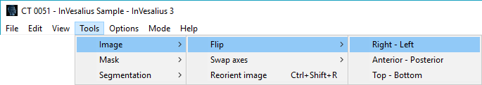
Fig. 28 Menu to activate flip image tool.#
Fig. 29 and Fig. 30 show a comparison between the input image and the flipped image. All other orientations are also modified when the image is flipped.
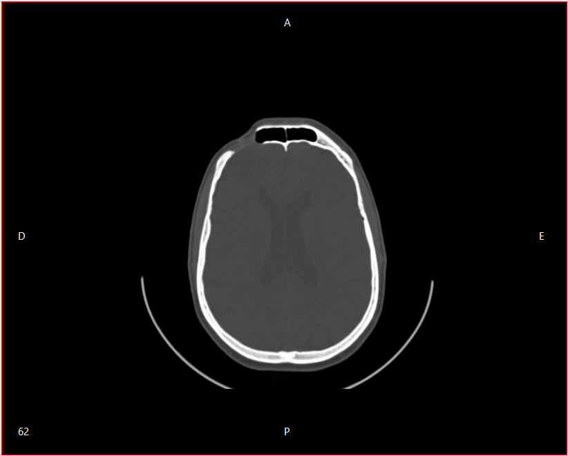
Fig. 29 The image before mirroring.#
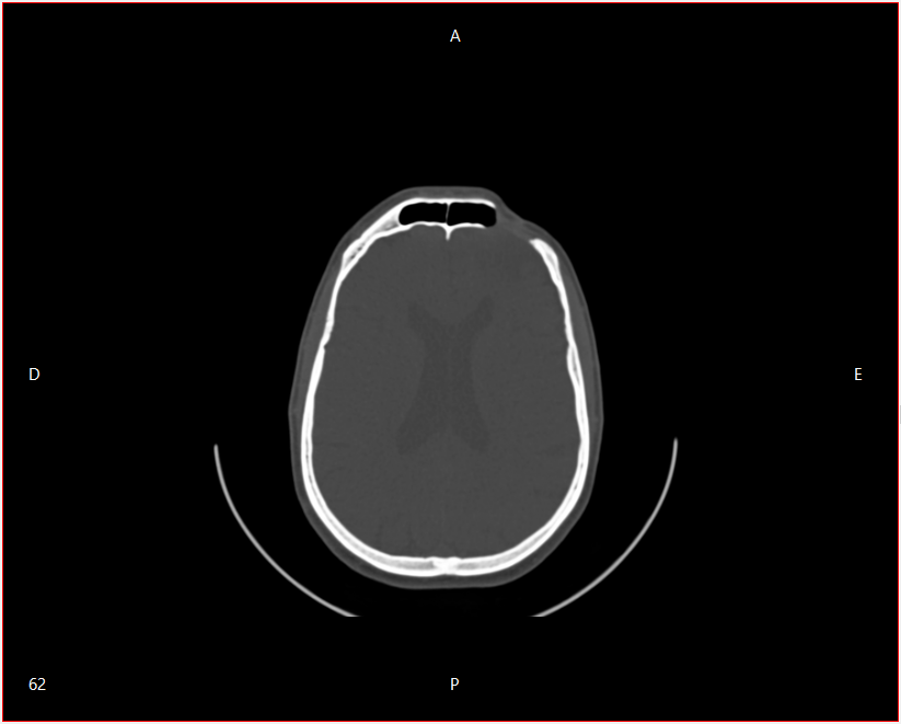
Fig. 30 The image after axial mirroring.#
Swap Axes#
The swap axes tool changes the image orientation, in the case that the image has been wrongly imported. To perform this, select the Tools menu, click Image, then Swap Axes and click on one of the following options (Fig. 31):
From Right-Left to Anterior-Posterior
From Right-Left to Top-Bottom
From Anterior-Posterior to Top-Bottom
The Fig. 32 and Fig. 33 show an example of an image with inverted axes.
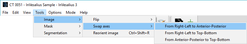
Fig. 31 Menu to activate swap image tool.#
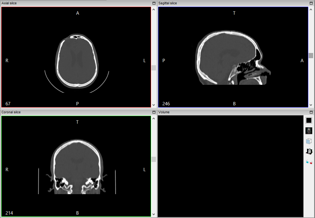
Fig. 32 Images before swap axes - from Anterior-Posterior to Top-Bottom.#
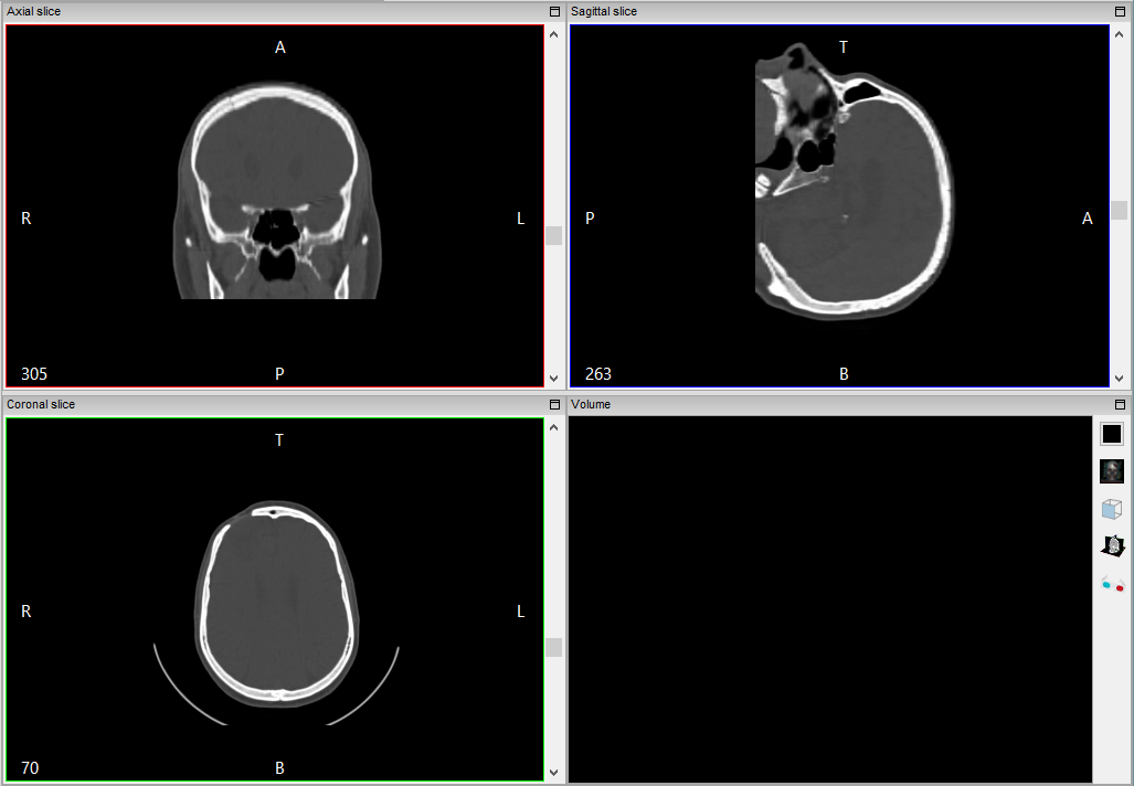
Fig. 33 Images after swap axes - from Anterior-Posterior to Top-Bottom.#
Reorient Image (Rotate)#
If it is necessary to align the image with a certain point of reference, e.g. anatomical marker, use the reorient image tool. To open this tool, select the Tools menu, click Image, then Reorient Image (Fig. 34).
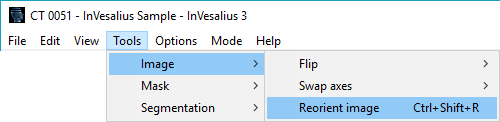
Fig. 34 Menu to activate reorient image tool.#
When this tool is activated, a window is opened (Fig. 35) showing orientation and by how many degrees the image was rotated.
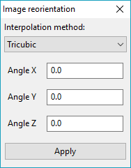
Fig. 35 Window that shows the reorientation image parameters.#
To start reorienting the image, define the interpolation method that will be applied after rotation, by default is tricubic interpolation. The interpolation options are:
Nearest Neighbour
Trilinear
Tricubic
Lanczos
Then, select the rotation point by keeping the left mouse button pressed between the two lines intersecting (Fig. 36) at one orientation, e.g. axial, coronal or sagittal, and drag to the desired point.
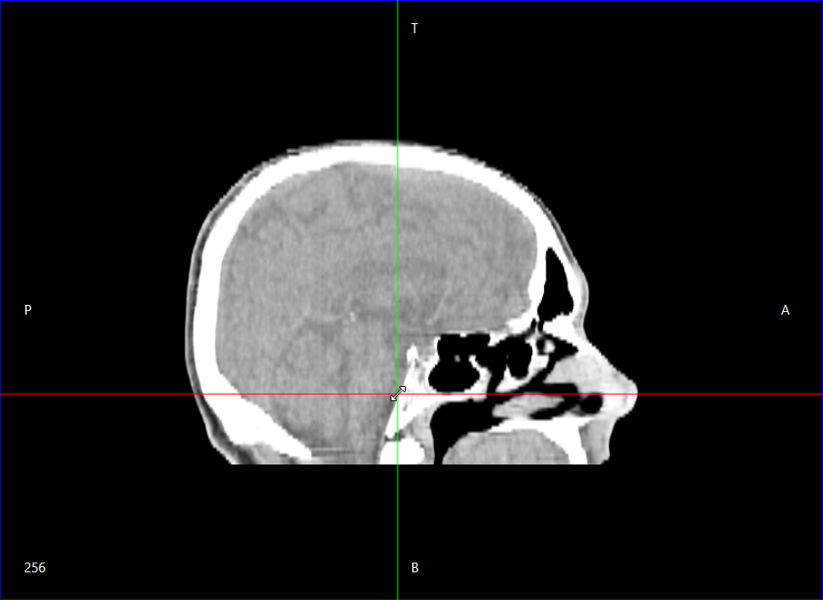
Fig. 36 Defining the axis of rotation of the image.#
To rotate the image, it is necessary to keep the left mouse button pressed and drag until the reference point or anatomical marker stays aligned with one of the lines (Fig. 37). After the image is in the desired position, click Apply in the parameter window (Fig. 35). This may take a few moments depending on the image size. Fig. 38 shows an image successfully reoriented.
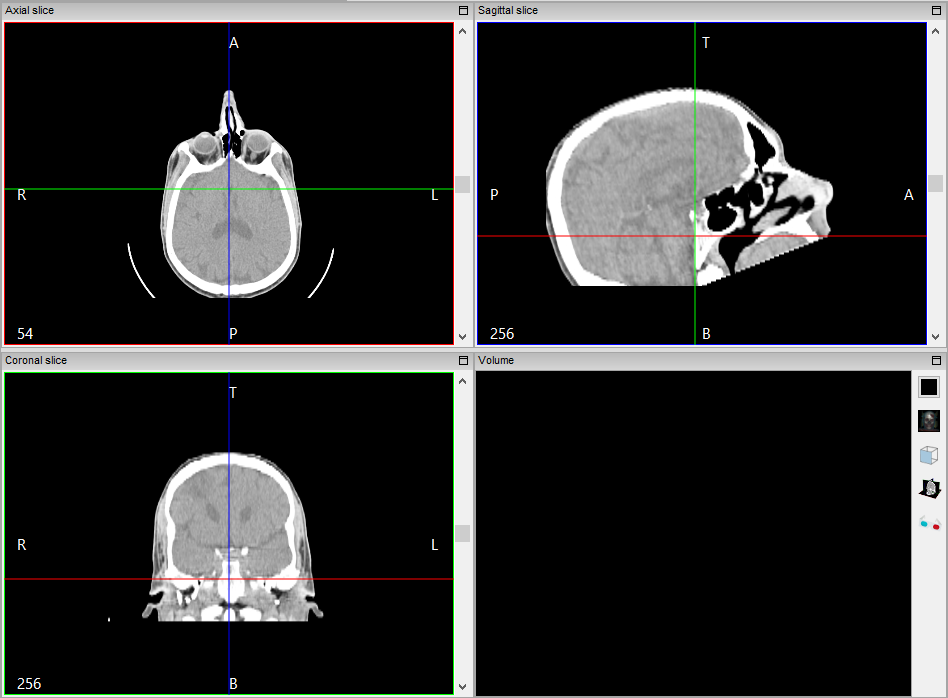
Fig. 37 Rotated image.#
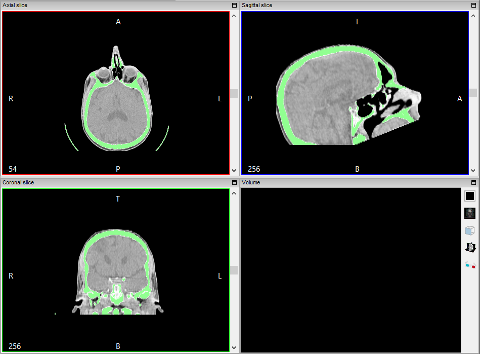
Fig. 38 Rotated image after reorientation is done.#
Image Manipulation (2D)#
Multiplanar Reconstruction#
When images are imported, InVesalius automatically shows its multiplanar reconstruction in the Axial, Sagittal and Coronal orientations, as well as a window for 3D manipulation, as seen in Fig. 39.
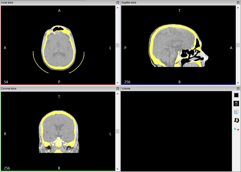
Fig. 39 Multiplanar reconstruction#
In addition to creating a multiplanar reconstruction, InVesalius segments an image. For example, soft tissue bones can be highlighted. The highlight is represented by the application of colors on a segmented structure so that the colors form a mask over an image highlighting the structure (Fig. 39).This is discussed in more detail in the following sections.
To hide the mask, use the data manager, located in the lower left corner of the screen. Select the Masks tab and click once using the left mouse button over the eye icon next to “Mask 1”, as shown in Fig. 40.
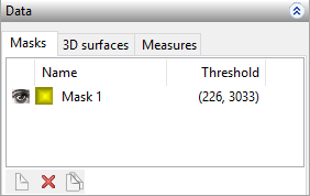
Fig. 40 Mask manager#
The eye icon disappears, and the colors of the segmentation mask are hidden (Fig. 41).
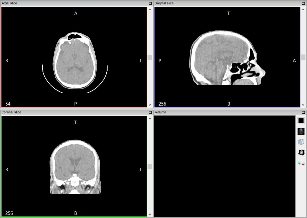
Fig. 41 Multiplanar reconstruction without segmentation mask#
Axial Orientation#
The axial orientation consists of cuts made transversally to the region of interest, i.e. parallel cuts to the axial plane of the human body. In Fig. 42, an axial image of the skull region is displayed.
Fig. 42 Axial slice#
Sagittal Orientation#
The sagittal orientation consists of cuts made laterally in relation to the region of interest, i.e. parallel cuts to the sagittal plane of the human body, which divides it into the left and right portions. In Fig. 43, a sagittal skull image is displayed.
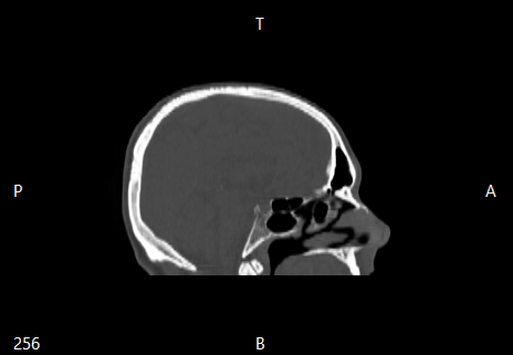
Fig. 43 Sagittal slice#
Coronal Orientation#
The coronal orientation is composed of cuts parallel to the coronal plane, which divides the human body into ventral and dorsal halves. In Fig. 44 is displayed a skull image in coronal orientation.
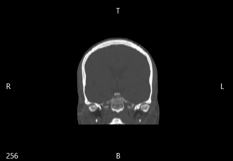
Fig. 44 Coronal slice#
Correspondence Between the Axial, Sagittal and Coronal Orientations#
To find out the common point of intersection of the images in different orientations, simply activate the “Slices cross intersection” feature with the shortcut icon located on the toolbar. See Fig. 45.

Fig. 45 Shortcut to show common point between different orientations.#
When the feature is activated, two cross-sections that intersect perpendicularly are displayed on each image (Fig. 46). The intersection point of each pair of segments represents the common point between different orientations.
To modify the point, hold down the left mouse button and drag. Automatically, the corresponding points will be updated in each image.
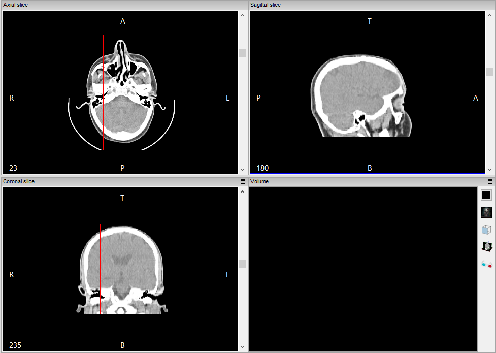
Fig. 46 Common point between differents orientations.#
To deactivate the feature, simply click on the shortcut again (Fig. 45). This feature can be used in conjunction with the slice editor (which will be discussed later).
Interpolation#
By default, the 2D images visualization is interpolated (Fig. 48. To deactivate this feature, select the View menu and select Interpolated slices (Fig. 47). It will then be possible to visualize each pixel individually as shown in Fig. 49.
This interpolation is for visualization purposes only, and does not directly influence segmentation or 3D surface generation.
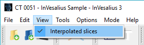
Fig. 47 Menu to disable and enable interpolation.#

Fig. 48 Interpolated image visualization.#
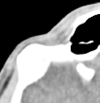
Fig. 49 Non-interpolated image visualization.#
Move#
To move an image on the screen, use the Move shortcut icon on the toolbar (Fig. 50). Click on the icon to activate, then with the left mouse button on the image, it to the desired direction. Fig. 51 shows a displaced (moved) image.

Fig. 50 Shortcut to move images.#
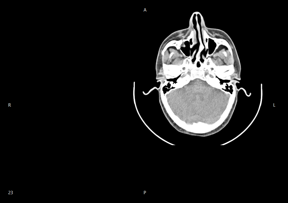
Fig. 51 Displaced image.#
Rotate#
Images can be rotated by using the Rotate shortcut on the toolbar (Fig. 52). To rotate an image, click on the icon and then with the left mouse button drag clockwise or anticlockwise as required.

Fig. 52 Shortcut to rotate images.#
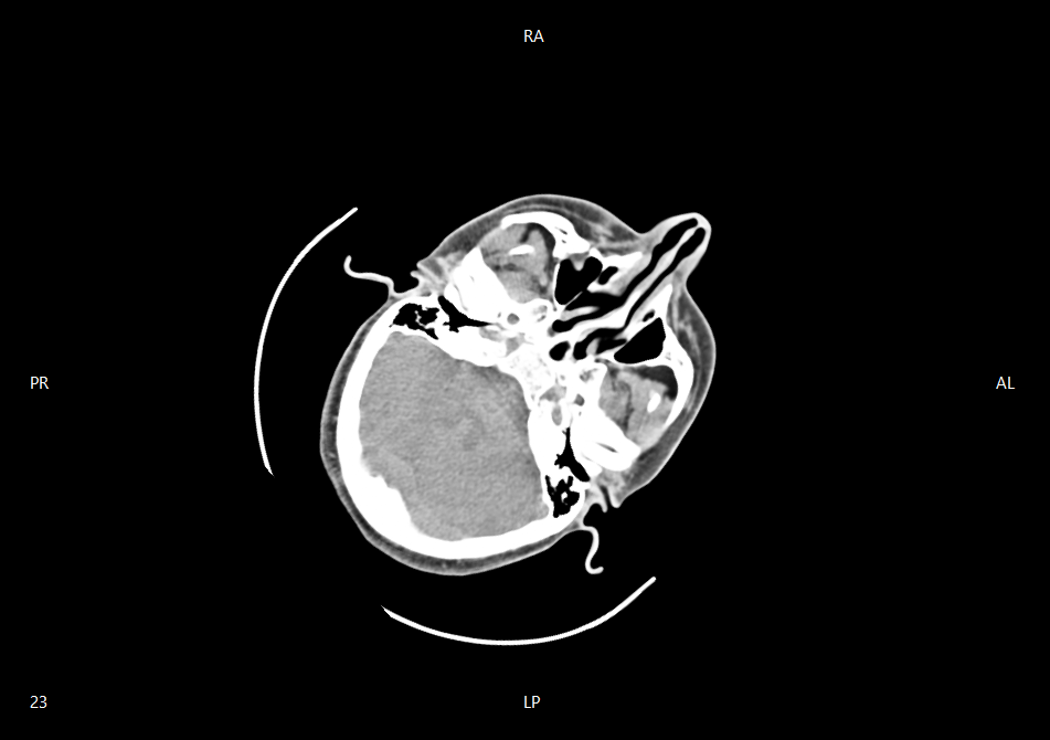
Fig. 53 Rotated image#
Zoom#
In InVesalius, there are different ways to enlarge an image. You can maximize the desired orientation window, apply zoom directly to the image, or select the region of the image to enlarge. Each of these methods is detailed below.
Maximizing Orientation Windows#
The main InVesalius window is divided into 4 sub-windows: axial, sagittal, coronal and 3D. Each of these can be maximized to occupy the entire area of the main window. To do this, simply left mouse click on the subwindow icon located in the upper right corner (Fig. 54). To restore a maximized window to its previous size, simply click the icon again.
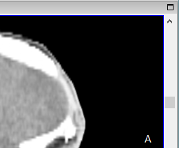
Fig. 54 Detail of a sub-window (Note the maximize icon in the upper right corner).#
Enlarging or Shrinking an Image#
To enlarge or shrink an image, click on the zoom shortcut icon in the toolbar (Fig. 55). Hold down the left mouse button on the image and drag the mouse up to enlarge or down to shrink.

Fig. 55 Zoom shortcut#
Enlarging an Image Area#
To enlarge a certain image area, click on the “Zoom based on selection” icon in the toolbar (Fig. 56). Position the mouse pointer at the origin point of the selection, click and hold the left mouse button and drag it to the end selection point to form a rectangle (Fig. 57). Once the left mouse button is released, the zoom operation will be applied to the selected region (Fig. 58).

Fig. 56 Zoom based on selection shortcut.#
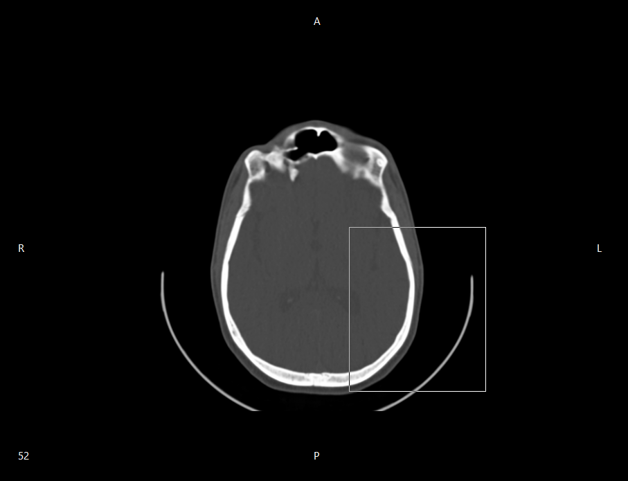
Fig. 57 Area selected for zoom.#
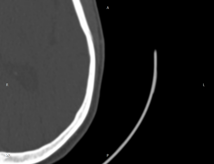
Fig. 58 Enlarged image.#
Brightness and Contrast (Windows)#
To improve image visualization, the window width and window level features can be used; these are more commonly known as brightness and contrast or window (for radiologists). With this feature, it is possible to set the range of the gray scale (window level) and the width of the scale (window width) to be used to display the images.
The feature can be activated by the “Brightness and Contrast” shortcut icon in the toolbar. See Fig. 59.

Fig. 59 Brightness and contrast shortcut#
To increase the brightness, hold down the left mouse button and drag horizontally to the right. To decrease the brightness, simply drag the mouse to the left. The contrast can be changed by dragging the mouse (with the left button pressed) vertically: up to increase, or down to decrease contrast.
To deactivate the feature, click again on the shortcut icon (Fig. 59).
Preset brightness and contrast patterns may be used with InVesalius. The table below lists some tissue types with their respective brightness and contrast values. To use the presets, position the mouse cursor over an image and right-click to open a context menu, then select Window width and level, and click on the preset option according to the tissue type, as shown in Fig. 60.
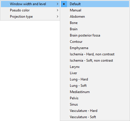
Fig. 60 Context menu for brightness and contrast selection#
Brightness and contrast values for some tissues
Tissue |
Brightness |
Contrast |
|---|---|---|
Default |
Exam |
Exam |
Manual |
Changed |
Changed |
Abdomen |
350 |
50 |
Bone |
2000 |
300 |
Brain |
80 |
40 |
Brain posterior fossa |
120 |
40 |
Contour |
255 |
127 |
Emphysema |
500 |
-850 |
Ischemia - Hard, non-contrast |
15 |
32 |
Ischemia - Soft, non-contrast |
80 |
20 |
Larynx |
180 |
80 |
Liver |
2000 |
-500 |
Lung - Hard |
1000 |
-600 |
Lung - Soft |
1600 |
-600 |
Mediastinum |
350 |
25 |
Pelvis |
450 |
50 |
Sinus |
4000 |
400 |
Vasculature - Hard |
240 |
80 |
Vaculature - Soft |
680 |
160 |
Pseudo Color#
Another feature to improve the visualization of the images is the pseudo color. This replaces gray levels by color, or by inverted gray levels. In the latter case, previously clear regions of the image become darker and vice versa.
To change the view using a pseudo color, position the mouse cursor over the image and right-click to open a context menu on it. When the menu opens, select the entry Pseudo color, and then click on the desired pseudo color option, as shown in Fig. 61.
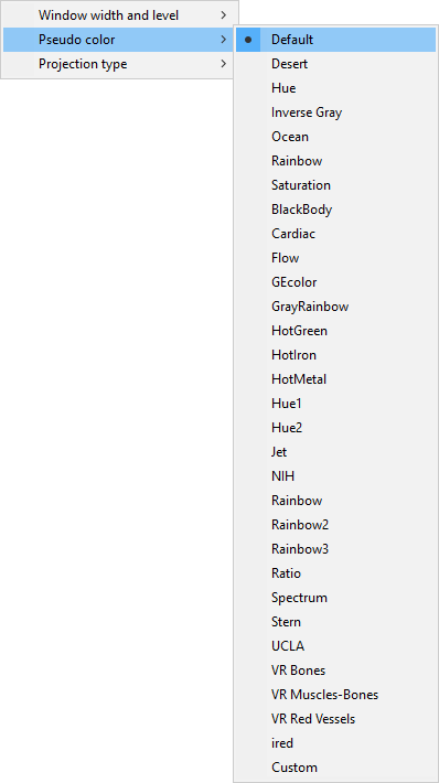
Fig. 61 Pseudo color#
Figures below demonstrate the various pseudo color options available.
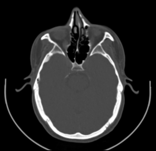
Fig. 62 Default pseudo color.#
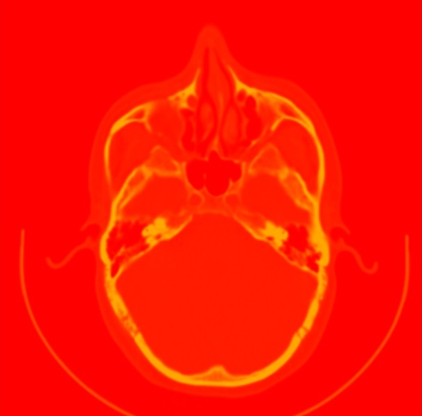
Fig. 63 Desert pseudo color.#
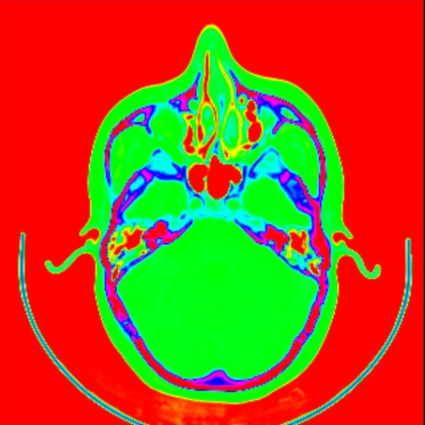
Fig. 64 Hue pseudo color.#
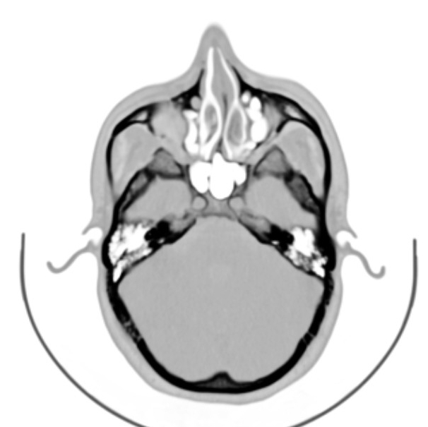
Fig. 65 Inverse pseudo color.#
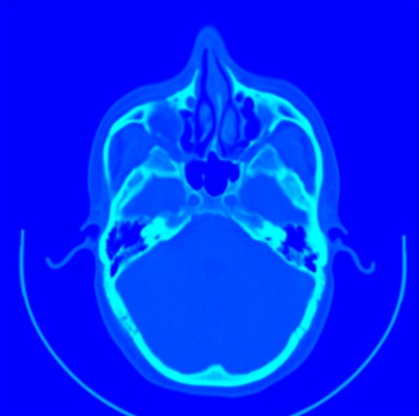
Fig. 66 Ocean pseudo color.#
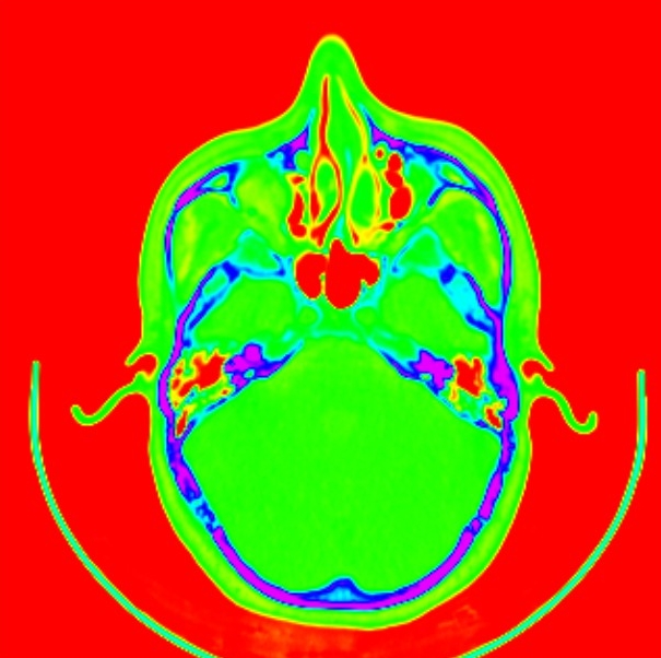
Fig. 67 Rainbow pseudo color.#
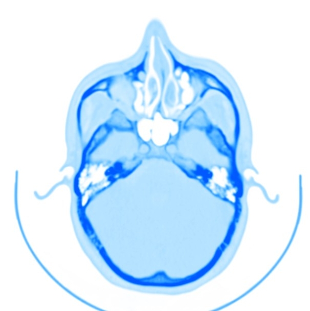
Fig. 68 Saturation pseudo color.#
Projection Type#
It is possible to change the projection type of the 2D images, in addition to the normal mode, InVesalius has six types of projections that can be accessed as follows: Place the mouse over the image and right-click to open a context menu on it. When the menu opens, select the projection type option, and then click on the desired projection option, as shown in the Fig. 69.
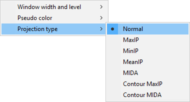
Fig. 69 Projection type menu#
Normal#
Normal mode is the default view, showing the unmodified image as it was when acquired or customized previously with either brightness and contrast or pseudo color. Normal mode is shown below in Fig. 70.
Fig. 70 Normal projection#
MaxIP#
MaxIP is also known as MIP (Maximum Intensity Projection). MaxIP selects only voxels that have maximum intensity among those visited as shown in Fig. 71. According to the amount of, or “depth” of MaxIP, each voxel is visited in order of overlap, for example, to select MaxIP of the pixel (0, 0) consisting of 3 slices it is necessary to visit pixel (0, 0) of slices (1, 2, 3) and select the highest value.
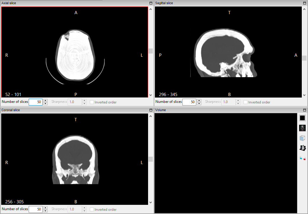
Fig. 71 MaxIP projection#
As shown in Fig. 72, the number of MaxIP images is set at the bottom of each orientation image.

Fig. 72 Selection the amount of images that composes the MaxIP or MIP#
MinIP#
Unlike MaxIP, MinIP (Minimum Intensity Projection) selects only the voxels that have minimal intensity among those visited, as shown in Fig. 73. The image number selection comprising the projection is made at the bottom of each orientation image as shown in Fig. 72.
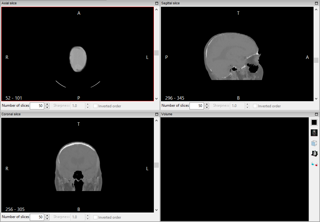
Fig. 73 MinIP projection#
MeanIP#
The MeanIP (Mean Intensity Projection) technique which is shown in the Fig. 74 composes the projection by averaging voxels visited in the same way as the MaxIP and MinIP methods. It is also possible to define how many images will compose the projection at the bottom of the image of each orientation as shown in Fig. 72.
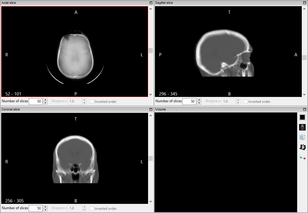
Fig. 74 MeanIP projection#
MIDA#
The MIDA (Maximum Intensity Difference Accumulation) technique projects an image taking into account only voxels that have local maximum values. From each pixel a ray is simulated towards the volume, with each voxel being intercepted by each ray reaching the end of the volume. Each of the voxels visited has its accumulated value, but are taken into account only if the value is greater than previously visited values. Like MaxIP, one can select how many images are used to accumulate the values. Fig. 75 shows an example of MIDA projection.
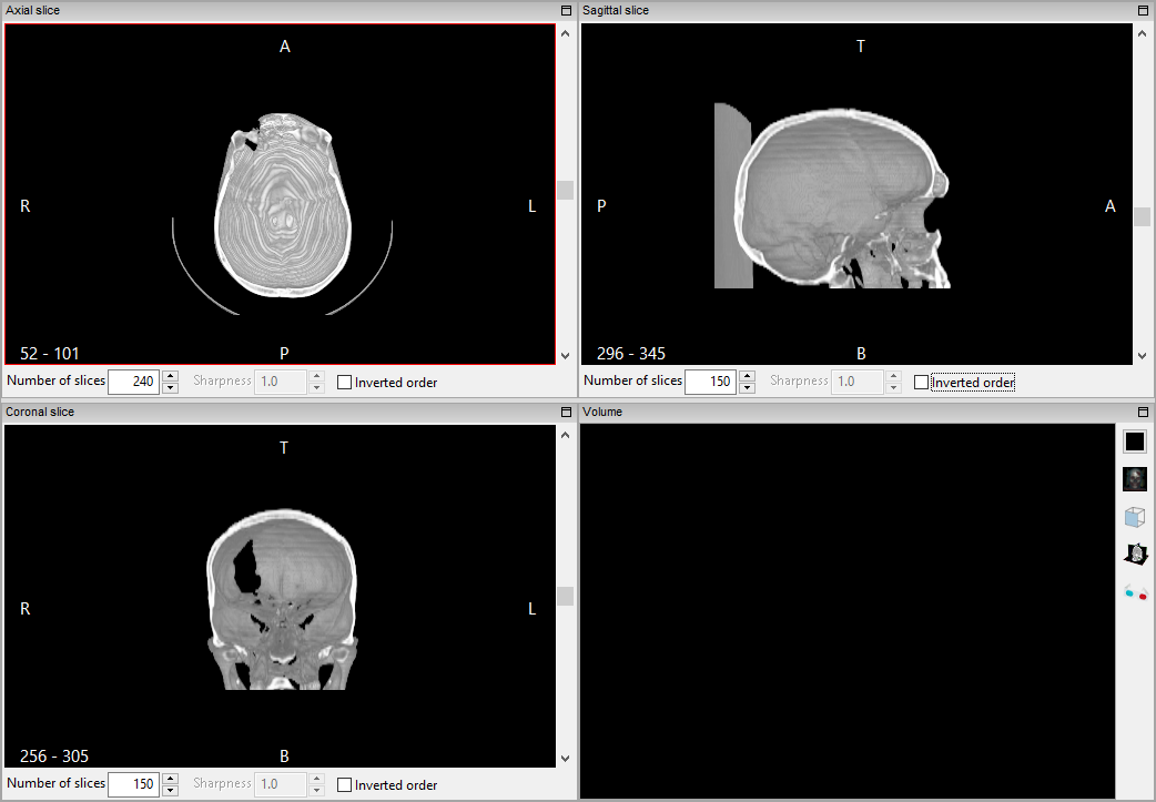
Fig. 75 MIDA projection#
As Fig. 76 shows, it is possible to invert the order that the voxels are visited by selecting the Inverted order option in the lower corner of the screen.
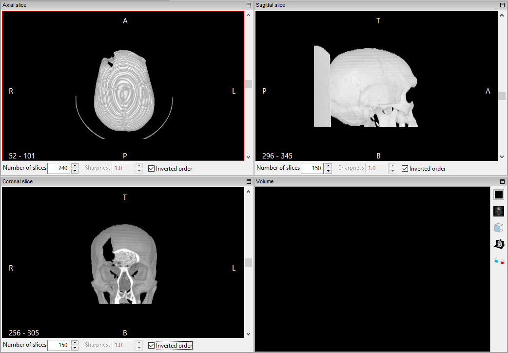
Fig. 76 Inverted order MIDA projection#
Contour MaxIP#
The Contour MaxIP function consists of visualizing contours present in the projection generated with MaxIP technique (MaxIP). An example is presented in Fig. 77.
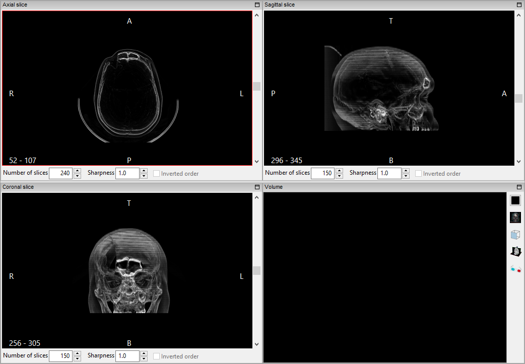
Fig. 77 Contour MaxIP projection#
Contour MIDA#
The Contour MIDA function consists of visualizing contours present in the projection generated with the MIDA technique (MIDA). Like MIDA, you can reverse the order that the volume is visited, as shown in Fig. 78.
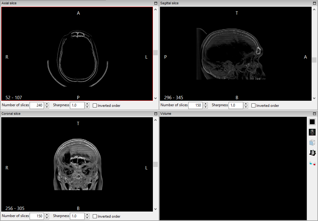
Fig. 78 Contour MIDA projection#
Segmentation#
To select a certain type of tissue from an image, it is used the segmentation feature at InVesalius.
Threshold#
When using the thresholding segmentation technique, only the pixels whose intensity is inside the threshold range defined by the user are detected. The threshold is defined by two values, the initial (minimum) and final (maximum) threshold.
In thresholding segmentation technique only the pixels whose intensity is inside threshold range defined by the user. The Threshold is defined by two numbers, the initial and final thresholds, also known as the minimum and maximum thresholds.
Thresholding segmentation is located on the InVesalius left-panel, item 2. Select region of interest (Fig. 79).
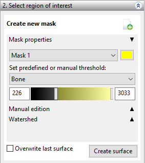
Fig. 79 Select region of interest -threshold.#
Before starting a segment, it is necessary to configure a mask. A mask is an image over to examine an image where the selected regions are colored (Fig. 80).
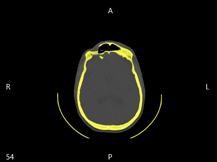
Fig. 80 Mask - selected region in yellow.#
To change the threshold, use the image greyscale control (Fig. 81). Move the left sliding control to change the initial threshold. Move the right sliding control to change the final threshold. It is also possible to input the desired threshold values in the text boxes in the left and right side of the thresholding control. The mask will be automatically updated when the thresholding values are changed, showing in color the pixels inside the thresholding range.
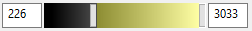
Fig. 81 Selecting pixels with intensity between 226 and 3021 (Bone).#
It is also possible to select some predefined thresholding values based on some type of tissues, like those displayed in Fig. 82. Just select the desired tissue and the mask will automatically update.
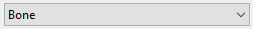
Fig. 82 Selection list with some predefined thresholding values.#
The table below shows thresholding values according to tissues and materials. The table indicates images obtained from medical tomographs. The range of gray values from images obtained from odontological tomographs is greater and non-regular. Thus, it is necessary to use sliding controls (Fig. 81) to adjust the thresholding values.
Table - Predefined thresholding values to some materials
Material |
Initial threshold |
Final threshold |
|---|---|---|
Bone |
226 |
3021 |
Compact Bone (Adult) |
662 |
1988 |
Compact Bone (Child) |
586 |
2198 |
Custom |
User Def. |
User Def. |
Enamel (Adult) |
1553 |
2850 |
Enamel (Child) |
2042 |
3021 |
Fat Tissue (Adult) |
-205 |
-51 |
Fat Tissue (Child) |
-212 |
-72 |
Muscle Tissue (Adult) |
-5 |
135 |
Muscle Tissue (Child) |
-25 |
139 |
Skin Tissue (Adult) |
-718 |
-177 |
Skin Tissue (Child) |
-766 |
-202 |
Soft Tissue |
-700 |
225 |
Spongial Bone (Adult) |
148 |
661 |
Spongial Bone (Child) |
156 |
585 |
To create a new mask, click Create new mask (Fig. 83). Then, click Select region of interest.

Fig. 83 Button to create a new mask.#
After clicking on this button, a dialog will be shown (Fig. 84). Select the desired threshold and click on Ok.
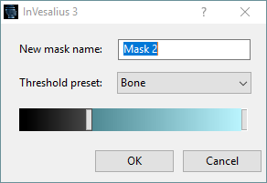
Fig. 84 Creating a new mask.#
After segmentation, it is possible to generate a corresponding 3D surface. The surface is formed by triangles. The following chapter will give more details about surfaces.
Click on the Create surface button (Fig. 85) to create a new surface. If there is a surface created, previously you may overwrite it with the new one. To do this, select the option Overwrite last surface before creating the new surface.
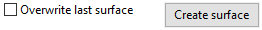
Fig. 85 Create surface button.#
After a few moments the surface will be displayed at the 3D visualization window of InVesalius (Fig. 86).
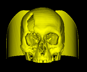
Fig. 86 3D surface.#
Manual Segmentation (Image edition)#
Thresholding segmentation may not be efficient in some cases since it is applied to the whole image. Manual segmentation may be used to segment only an isolated region. Manual segmentation also allows users to add or remove some image regions from the segmentation. To use it, click on Manual edition (Fig. 87) to open the manual segmentation panel.

Fig. 87 Icon to open the Manual segmentation panel.#
Fig. 88 shows the Manual segmentation panel.
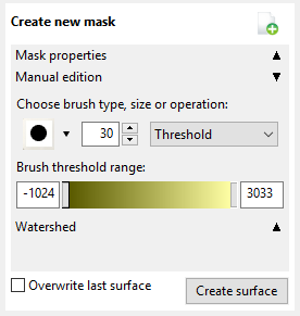
Fig. 88 Manual segmentation panel.#
There are two brushes used for segmentation: a circle and a square. Click on the triangle icon (see Fig. 89) to show brush types, then click on the desired brush.

Fig. 89 Brush types.#
Brush sizes can also be adjusted, as shown in Fig. 90.

Fig. 90 Adjusting the brush size.#
The following are available options when using brushes in InVesalius:
Draw: for adding a non-selected region to the segmentation;
Erase: for removal of a non-selected region;
Threshold: applies the thresholding locally, adding or removing a region inside or outside the threshold range.
Fig. 91 shows the available brush operations.
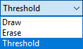
Fig. 91 Brush operations.#
Fig. 92 shows an image with noise caused by the presence of a dental prosthesis. Note the rays emerging from the dental arch: the thresholding segments the noise since its intensity is inside the threshold of bone.
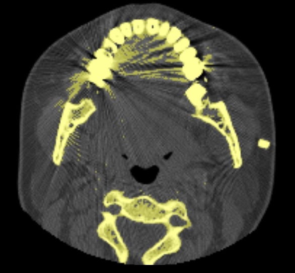
Fig. 92 Noisy image segmented with threshold.#
Fig. 93 shows a surface created from that segmentation.
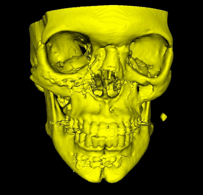
Fig. 93 Surface generated from noisy image.#
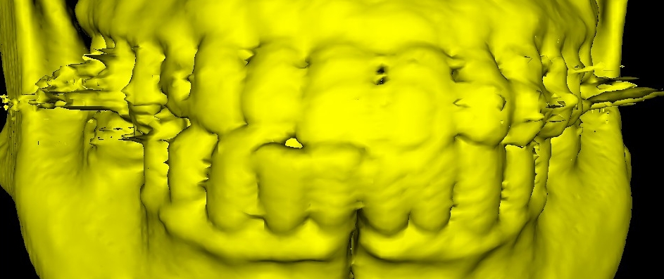
Fig. 94 Zoom in the noisy area.#
In such cases, use the manual segmentation with the erase brush. Keep the left mouse button pressed while dragging the brush over the region to be removed (in mask).
Fig. 95 shows the image from Fig. 92 after.
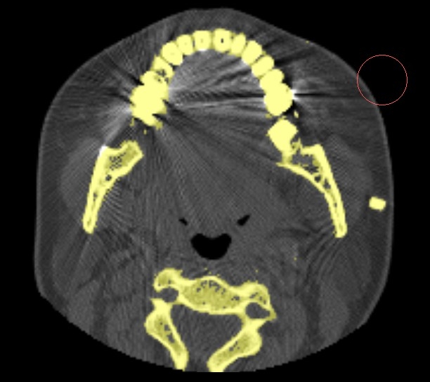
Fig. 95 After removing the noise.#
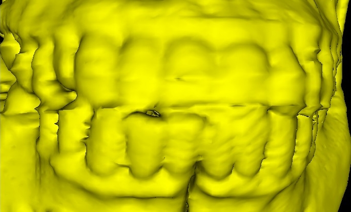
Fig. 96 Surface generate after removing the noise.#
A surface can be generated after manual segmentation (Fig. 96). Since it was used in the manual segmentation procedure, when clicking on Create surface button, a dialog (Fig. 97) will be opened to select if the surface is created with the method Binary (blocky) or Context aware smoothing (smoother).
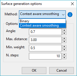
Fig. 97 Surface creation methods.#
Watershed#
In watershed segmentation, the user demarcates objects and background detail. This method treats the image as watershed (hence the name) in which the gray values (intensity) are the altitudes, forming valleys and mountains. The markers are water source. The waters fill the watershed until the waters gather together, thus distinguishing a background from an object. To use Watershed segmentation, click on Watershed to open the watershed panel (Fig. 98).
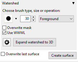
Fig. 98 Watershed segmentation panel.#
Before segmenting to with Watershed, it is recommended to clean the mask (see Mask Cleaning).
To insert a marker (object or background), a brush is used, similar to manual segmenting. You can use a circle or square brush and set its size.
Select brush operations from the following:
Object: to insert object markers;
Background: to insert background markers (not object);
Delete: to delete markers.
The option Overwrite mask is used when the user wants the result of watershed segmentation to overwrite the existing segmentation. The option Use WWWL is used to make watershed take into account the image with the values of window width and window level (not the raw image) which may result in better segmentation.
Click on the button on the left side of the panel (Fig. 99) to access more watershed configurations. This button will open a dialog (Fig. 100). The method option allows choosing the Watershed algorithm to be used to segment. It may be the conventional Watershed or Watershed IFT, which is based on the IFT (Image Forest Transform) method. In some cases, like brain segmentation, the Watershed IFT may have a better result.
The connectivity option refers to the pixel neighbourhood (4 or 8 when in 2D, or 6, 18 or 26 when in 3D). Gaussian sigma is a parameter used in the smoothing algorithm (the image is smoothed before the segmentation to remove the noise and get better results). The greater this value, the smoother the image will be.

Fig. 99 Button to open the Watershed configuration dialog.#
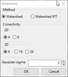
Fig. 100 Watershed configuration dialog.#
Normally the Watershed is applied only in one slice, not in the whole image. After adding the markers is possible to apply the watershed to the whole image by clicking on the button Expand watershed to 3D. Fig. 101 shows the result of watershed segmentation in a slice (2D) of brain image.
Fig. 102 shows the segmentation expanded to the whole image (3D).
Fig. 101 also shows the object markers (in light green), the background markers (in red) and the segmentation mask (in green) overlaying the selected regions (result).
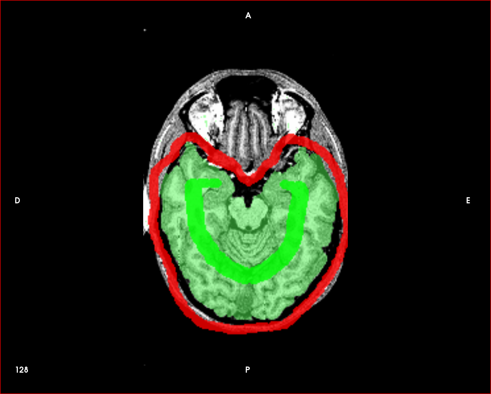
Fig. 101 Watershed applied to a slice.#
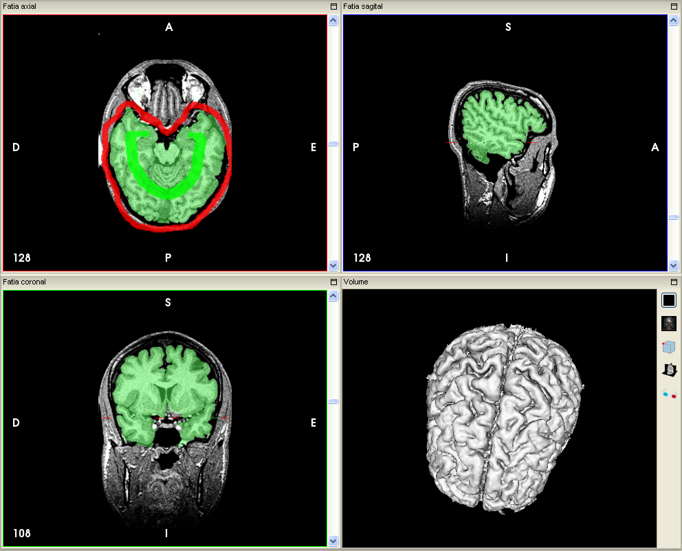
Fig. 102 Brain segmentation using the watershed method applied to the whole image (3D).#
Region Growing#
Region growing tool is accessed in the menu Tools, Segmentation, Region growing (Fig. 103). Before segmenting, select if the operation is in 2D - Actual slice or 3D — All slices. It is also necessary to select the connectivity: 4 or 8 to 2D or 6, 18 or 26 to 3D. It’s also necessary to select the method, which may be Dynamic, Threshold, or Confidence Fig. 104.
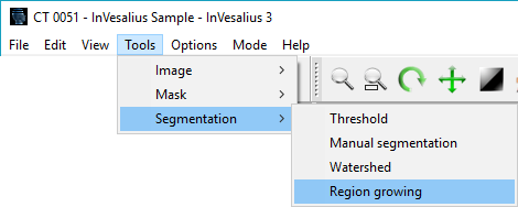
Fig. 103 Menu to access the region growing segmentation segmentation tool.#
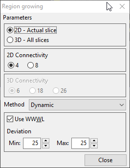
Fig. 104 Dialog to configure the parameters of region growing segmentation tool.#
This segmentation technique starts with a pixel (indicated by the user left-clicking with the mouse). The selection expands by analyzing the neighborhood of the selected pixels and including those of a given set of qualities. Each region-growing method has a different condition of selection:
Dynamic: Uses the value of the pixel clicked by the user. Then every connected pixel inside the lower (min) and the upper (max) range deviation are selected. The option Use WWWL is default and takes into account the image with window width and window level applied not the raw one (Fig. 105).
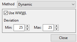
Fig. 105 Dynamic method parameters.#
Threshold: This method selects the pixels whose intensity are inside the minimum and maximum threshold (Fig. 106).
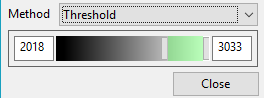
Fig. 106 Adjust the threshold.#
Confidence: This method starts by calculating the standard deviation and the mean value of the pixel selected by the user and its neighbourhood. Connected pixels with value inside the range (given by the mean more and less the standard deviation multiplied by the Multiplier parameter). It then calculates the mean and the standard deviation from the selected pixels, then carries out the expansion. This process is repeated according to the Iterations parameter. Fig. 107 shows the parameters for this method.
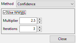
Fig. 107 Confidence parameter.#
Mask#
Boolean Operations#
After segmenting, some boolean operations can be performed between masks. The boolean operations supported by InVesalius are:
Union, perform union between two masks;
Difference, perform difference from the first mask to the second one;
Intersection, keeps what is common in both masks.
Exclusive disjunction (XOR): keeps the regions of the first mask which are not in the second mask and regions from the second mask which are not in the first mask.
To use this tool, go to the Tools, menu, select Mask, and then Boolean operations as shown in Fig. 108. Select the first mask, the operation to be performed and the second mask as shown in Fig. 109 then click OK.
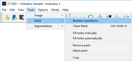
Fig. 108 Menu to open boolean operations tool.#
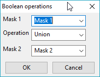
Fig. 109 Boolean operations tool.#
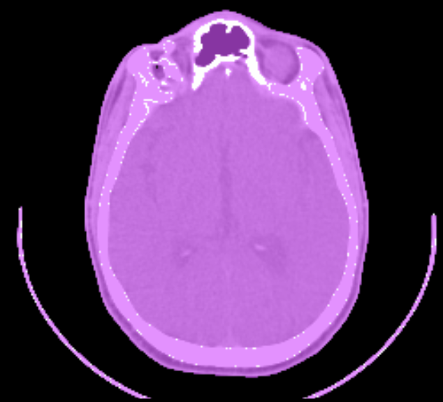
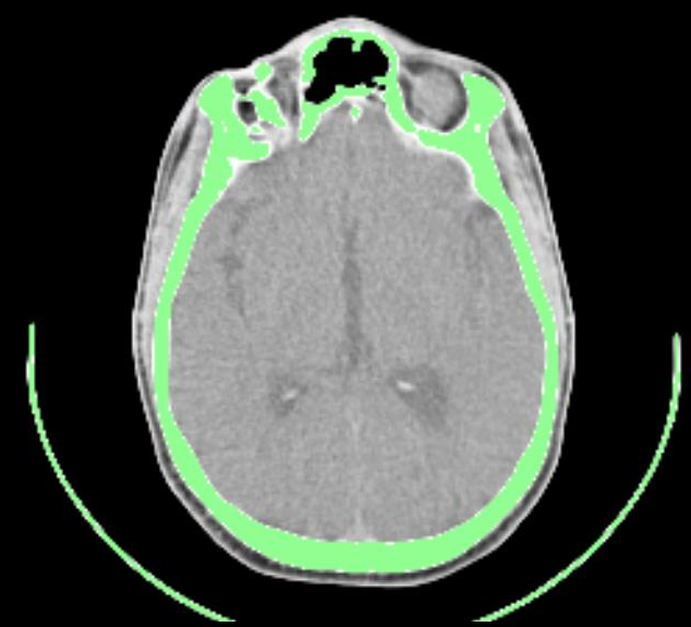
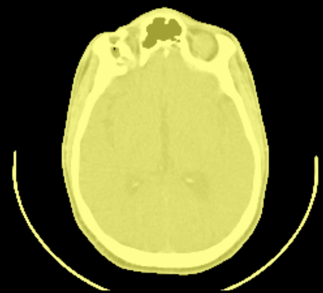
Figures below show some examples of boolean operations.
Mask Cleaning#
A mask can be cleaned, as shown in Fig. 110. This is recommended before inserting Watershed markers. This tool is located on the Tools menu. Select Mask, then Clean mask, or use the shortcut CTRL+SHIFT+A.
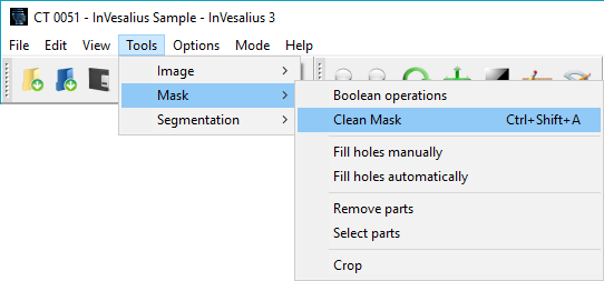
Fig. 110 Mask cleaning#
Fill Holes Manually#
Segmentation may leave some unwanted holes. It’s recommended to fill them because the surface generated from this mask may have some inconsistencies. To do this, access the menu Tools, Mask, Fill holes manually (Fig. 111). A dialog window will be shown (Fig. 112) to configure the parameters.
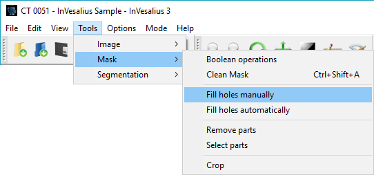
Fig. 111 Menu to access the tool to fill holes manually.#
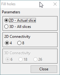
Fig. 112 Dialog to configure the parameters of Fill holes manually tool.#
It is possible to fill hole on a mask slice (2D - Actual slice) or on all slices, selecting the option (3D - All slices). The connectivity may also be configured: 4 or 8 for 2D and 6, 18 and 26 for 3D.
After configuring the desired parameters, left-click on holes to fill them. Fig. 113 shows a mask with some holes and Fig. 114 the mask with the holes filled. Click on the close button or close the dialog to deactivate this tool.
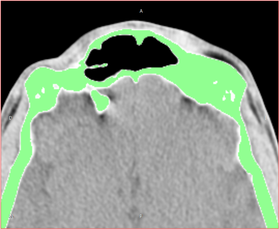
Fig. 113 A mask with holes.#

Fig. 114 A mask with filled holes.#
Fill Holes Automatically#
To open this tool, go to the Tools menu, select Mask then Fill holes automatically (Fig. 115). This will open a dialog to configure the parameters. This tool doesn’t require the user to click on the holes they desire to fill. This tool will fill the holes based on the max hole size parameter given in number of voxels (Fig. 116).
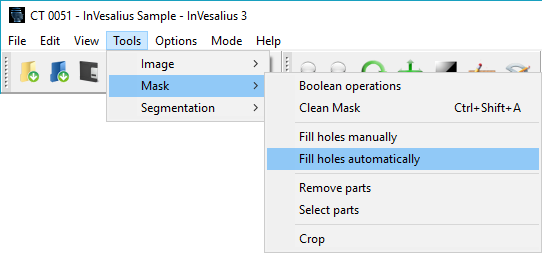
Fig. 115 Menu to open the Fill holes automatically tool.#
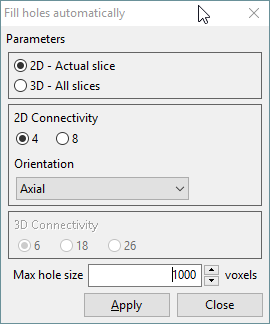
Fig. 116 Dialog to configure the parameters used to fill the holes.#
Holes can also be filled on a mask slice (2D - Actual slice) or on all slices, selecting the option (3D - All slices). The connectivity will thus be 4 or 8 to 2D and 6, 18 and 26 to 3D. If 2D, the user must indicate in which orientation window the holes will be filled.
After setting the parameters, click Apply. If the result is not suitable, set another hole size value or connectivity. Click Close to close this tool.
Remove Parts#
After generating a surface, it is recommended to remove the unwanted disconnected parts from a mask. This way, the surface generation will use less RAM and make the process quicker. To remove any unwanted parts, go to the Tools menu, select Mask and then Remove Parts (Fig. 117). A dialog will be shown to configure the selection parameters (Fig. 118).
It’s possible to select disconnected parts only on a mask slice (2D - Actual slice) or on all slices (3D - All slices); users may also configure the connectivity at the same time.
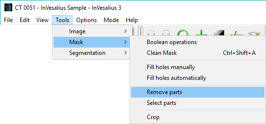
Fig. 117 Menu to open the Remove parts tool.#
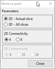
Fig. 118 Dialog to configure the parameters used in Remove parts.#
After selecting the desired parameters, click with the left-button of the mouse on the region you want to remove. Click Close to stop using this tool.
Select Parts#
To open the Select parts tool, access the Tools menu, select Mask then Select parts (Fig. 119). A dialog will be shown to configure the name of the new mask and the connectivity (6, 18 or 26).
To select a region, left-click on a pixel; multiple regions can be selected. The selected region(s) will be shown with a red mask. After selecting all the wanted regions, click OK to create a new mask with the selected regions. Fig. 121 shows a region selected in red. Fig. 122 shows the selected region in a new mask.
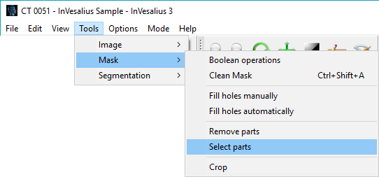
Fig. 119 Menu to open the Select parts tool.#
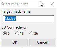
Fig. 120 Dialog to configure the parameters of Select parts tool.#
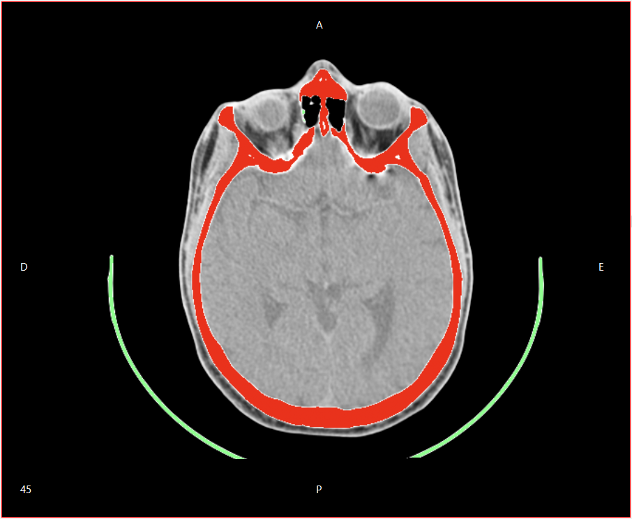
Fig. 121 Example of mask region selection.#
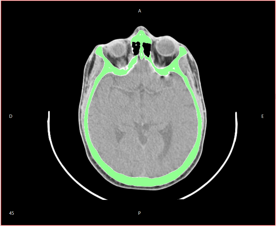
Fig. 122 Final image with only the selected region#
Crop#
The crop tool allows users to select and use a specific section of image of interest. This may reduce the amount of information needed to be processed when generating a surface. To open, access the Tool menu, then Mask and Crop (Fig. 123).
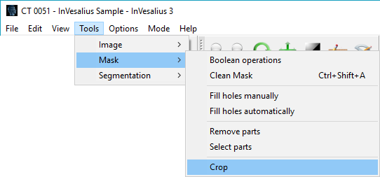
Fig. 123 Menu open the Crop tool.#
A box allowing for the selection of a specific area will then be displayed.
Surface (Triangle mesh)#
InVesalius generates 3D surfaces based on image segmentation. A surface is generated using the marching cubes algorithm by transforming voxels from the stacked and segmented images to polygons (triangles in this case).
The controls to configure a 3D surface are accessible on the left panel, under 3. Configure 3D surface, Surface properties you have the controls to configure a 3D surface (Fig. 124).
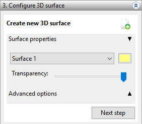
Fig. 124 3D surface configuration.#
Creating 3D Surfaces#
News surfaces can be created using an already segmented mask. To do so, on the left panel under 3. Configure 3D surface, click on the button shown in Fig. 125.
Fig. 125 Button to create a 3D surface.#
After clicking this button, a dialog will be shown (Fig. 126). This dialog allows for the configuration of the 3D surface created, including setting the quality of the surface, filling surface holes whilst keeping the largest connected region of the surface intact.
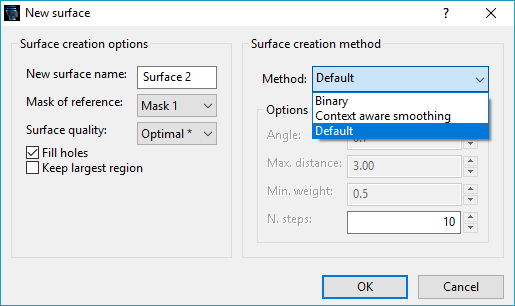
Fig. 126 3D surface creation dialog.#
The keep largest region option may be used, for instance, to remove the tomograph supports. Figures display a surface created with Keep the largest region and Fill holes activated, whereas Figures display the surface created without activating that options. Note the tomograph support and the holes.
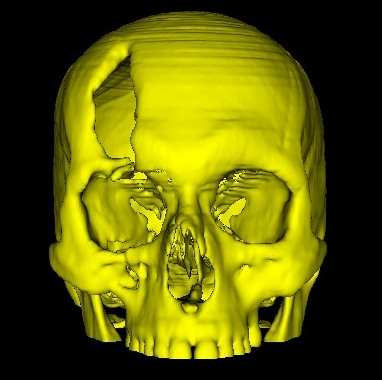
Fig. 127 Surface created with Keep the largest region and Fill holes activated (front).#
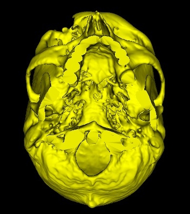
Fig. 128 Surface created with Keep the largest region and Fill holes activated (bottom).#
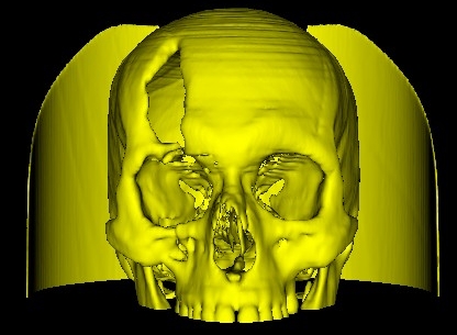
Fig. 129 Surface created without activating Keep the largest region and Fill holes (front).#
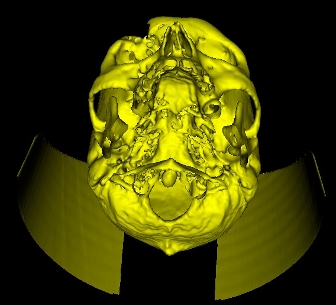
Fig. 130 Surface created without activating Keep the largest region and Fill holes (bottom).#
The Surface creation method item has the following options: Binary, Context aware smoothing and Default. Figures show an example of surface created using each of these 3 methods.
The Binary method takes as input the segmentation mask which is binary, where selected regions have value 1 and non-selected have value 0. As it is binary, the surface generated has a blocky aspect, mainly in high-curvature areas, appearing staircases.
Context aware smoothing starts generating the surface using Binary, then uses another algorithm in order to smooth the surface to avoid staircase details. This method has 4 parameters presented below.
The angle parameter is the angle between 2 adjacent triangles. If the calculated angle is greater than the angle parameter, the triangle will be considered a staircase triangle and will be smoothed. The angle parameter ranges from 0 to 1, where 0 is 0° and 1 is 90°. The Max distance is the maximum distance that a non-staircase triangle may be from a staircase triangle to be considered to be smoothed. Non-staircase triangles with distance greater than Max distance also will be smoothed, but the smoothing will be determined by the Min. weight parameter. This parameter ranges from 0 (without smoothing) to 1 (total smoothing). The last parameter, N.steps, is the number of times the smoothing algorithm will be run. The greater this parameter the smoother the surface will be.
The Default method is enabled only when thresholding segmentation was used without any manual modification to the mask. This method does not use the mask image, but the raw image, and generates a smoother surface.
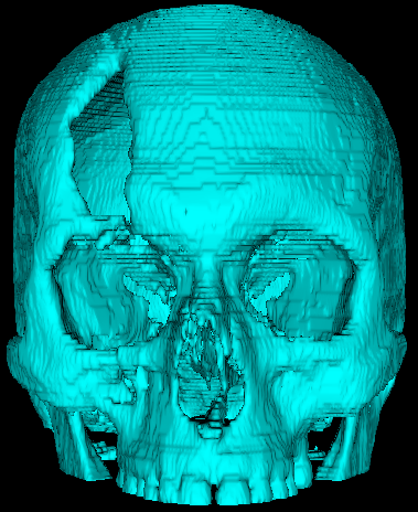
Fig. 131 Surface generated with Binary.#
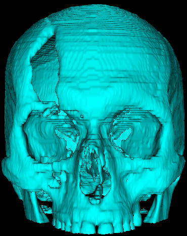
Fig. 132 Surface generated with Context aware smoothing.#
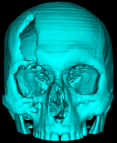
Fig. 133 Surface generated with Default.#
Transparency#
The Transparency function allows for the displaying of a surface transparently. To do so, select the desired surface from the list of surfaces in the item 3. Configure 3D surface, Surface properties (Fig. 134).
Fig. 134 Surface selection.#
Then, to set the level of surface transparency, use the sliding control shown in Fig. 135; the more to the right, the more transparent the surface will be.
Fig. 135 Selection of surface transparency.#
Fig. 136 shows 2 surfaces: the external surface in green has some level of transparency which permits seeing the internal surface in yellow.
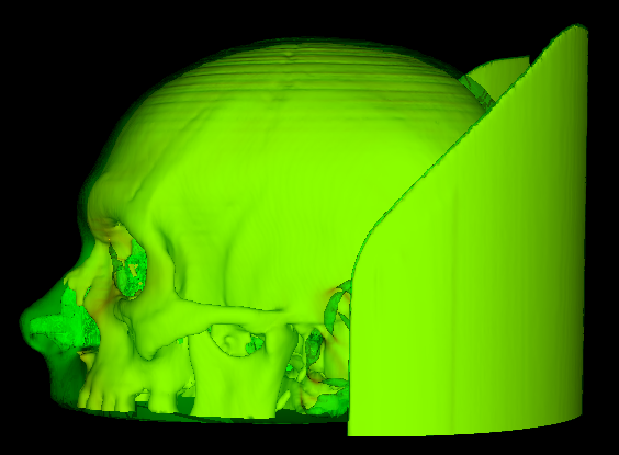
Fig. 136 Surface with transparency.#
Color#
Surface colors can be altered by selecting the surface (Fig. 134), and clicking on the colored button on the right of the surface selection list. Fig. 137 displays this button, inside item 3. Configure 3D surface, Surface properties.

Fig. 137 Button to change surface color.#
A dialog will be shown (Fig. 138). Select the desired color and click on OK.
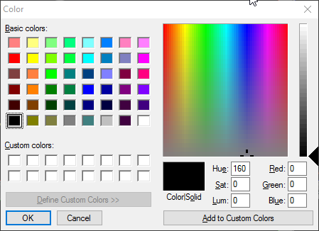
Fig. 138 Color dialog.#
Splitting Disconnected Surfaces#
To split disconnected surfaces, select 3. Configure 3D surface, Advanced options (Fig. 139).
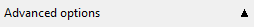
Fig. 139 Advanced options.#
The advanced options panel will be displayed (Fig. 140).
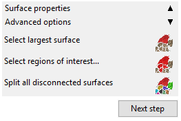
Fig. 140 Advanced options panel.#
Select Largest Surface#
The option Select largest surface selects, automatically, only surface with the greater volume. Click on the button illustrated in Fig. 141. This operation creates new a surface with only the largest surface.
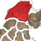
Fig. 141 Button to split the largest disconnected surface.#
As an example, the Fig. 142 shows a surface before Select the largest surface.
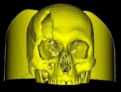
Fig. 142 Disconnected surfaces.#
Whereas the Fig. 143 shows the surface with the largest disconnected region separated.
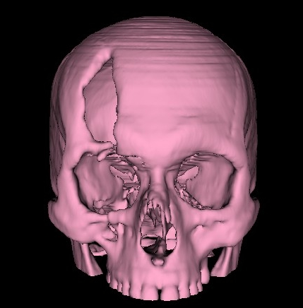
Fig. 143 Largest disconnected region separated.#
Select Regions of Interest#
Another selection option is Select regions of interest. To do this operation, click on the button illustrated in Fig. 144, then click on the desired disconnected surface regions you want to select. Next click on Select regions of interest. This operation will create a new surface with only the selected disconnected regions.
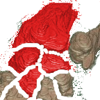
Fig. 144 Button to select the regions of interest.#
As an example, the Fig. 145 shows the surface created after the user selects the cranium and the right part of the tomograph support.
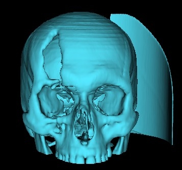
Fig. 145 Example of selected regions of interest.#
Split All Disconnected Surfaces#
Disconnected surface regions can also be split automatically. To do this, click on the button illustrated in Fig. 146.
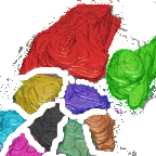
Fig. 146 Button to split all the disconnected regions surface.#
Fig. 147 shows an example.
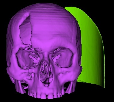
Fig. 147 Example of split all disconnected regions surface.#
Measures#
InVesalius has linear and angular measurements in 2D (axial, coronal and sagittal planes) and 3D (surfaces). It is thus possible to take measurements of volume and area on surfaces.
Linear Measurement#
To perform linear measurements, activate the feature by clicking on the shortcut shown below, located on the toolbar (Fig. 148).

Fig. 148 Shortcut to activate linear measurement.#
A linear measurement is taken between two points. With the feature enabled, click once on the image to set the starting point. Then position the mouse pointer on the end point and click once again. The measurement is performed and the result is automatically displayed on the image or surface
Fig. 149 shows a 2D linear measure in the axial orientation, and Fig. 150 shows another linear measure in 3D (surface).
Once you have made a 2D linear measurement, it can be edited by placing the mouse on one end, holding down the right mouse button and dragging it to the desired position.
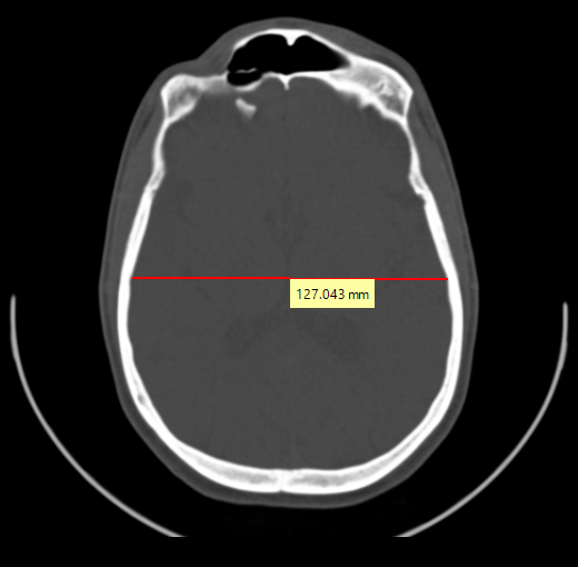
Fig. 149 Linear measure on image.#
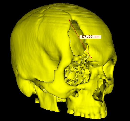
Fig. 150 Linear measure on surface.#
Note: The linear measurement is given in millimeters (mm).
Angular Measurement#
An angular measurement in 2D on a surface (3D) can be done by clicking on the shortcut shown in Fig. 151.

Fig. 151 Shortcut for angle measurement.#
To perform the angular measurement, it is necessary to provide the three points that will describe the angle to be measured, AB̂C. Insert the first point by clicking once to select point A. Insert point B (the vertex or “point” of the angle) by positioning the cursor and clicking once again. Repeat the same actions to determine the endpoint of the angle C. The resulting measurement is displayed on the image or surface.
Fig. 152 illustrates an angular measurement on a flat image; Fig. 153 illustrates an angular measurement on a surface.
In regard to 2D linear measurement, you can also edit the 2D angular measurement. Just position the mouse on one end, hold down the right mouse button and drag it to the desired position.
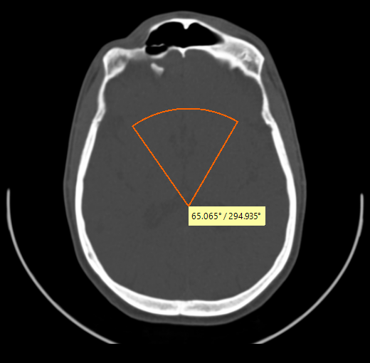
Fig. 152 Angular measurement.#
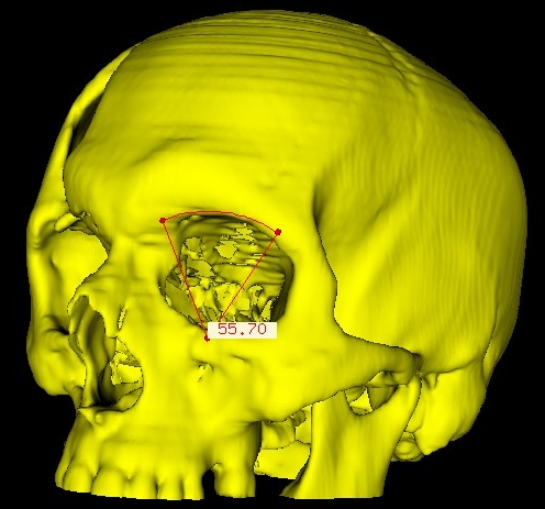
Fig. 153 Angular measurement on surface.#
Note: Angular measurement is shown in degrees (°)
Volumetric Measurement#
Volume and area measurements are made automatically when you create a new surface. These are displayed in the Surfaces 3D tab in the Data management panel, located in the bottom left corner of the screen, as illustrated in Fig. 154.
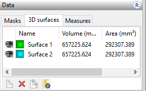
Fig. 154 Volumetric measurements.#
Note: Volume measurement is given in cubic millimeter (mm3), already the one of area in square millimeter (mm2).
Data Management#
We have previously shown how to manipulate surfaces, masks for segmentation and measurements. We can also show or hide and create or remove these elements in the Data management panel, located in the lower left corner of InVesalius. The panel is divided into 3 tabs: Masks, 3D Surfaces and Measurements, as shown in Fig. 155 Each tab contains features corresponding to the elements it refers to.
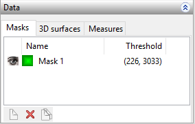
Fig. 155 Data management.#
In each tab, there is a panel divided into rows and columns. The first column of each line determines the visualization status of the listed element. The “eye” icon activates or deactivates the masks, surface or measurement displayed. When one of these elements is being displayed, its corresponding icon (as shown in Fig. 156) will also be visible.

Fig. 156 Icon indicating the elements visibility.#
Some operations may be performed with the data. For instance, to remove one element, first select its name, as shown in Fig. 157. Next, click on the shortcut shown in Fig. 158.
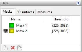
Fig. 157 Data selected.#

Fig. 158 Remove data.#
To create a new mask, surface or measurement, click on the shortcut shown in Fig. 159, provided that the corresponding tab is open.

Fig. 159 New data.#
To duplicate data, select data to be duplicated and click in the shortcut shown in Fig. 160.

Fig. 160 Duplicate data.#
Masks#
In the Name column, the mask’s color and name are shown. The Threshold column shows the value range used to create the mask. Fig. 155 shows an example.
3D Surface#
In the Name column, the surface’s color and name are shown. The Volume column shows the total surface volume. Finally, the Transparency column indicates the level of transparency for use for surface visualization. Fig. 161 shows an example.
Fig. 161 Surface manager.#
Import Surface#
We can also import STL, OBJ, PLY or VTP (VTK Polydata File Format) files into an active InVesalius project. To do so, click on the icon shown in Fig. 162, select the format of the corresponding file, (Fig. 163) and click Open.

Fig. 162 Shortcut to import surface.#
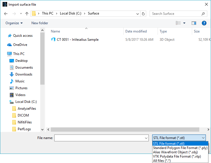
Fig. 163 Window to import surface.#
Measurements#
The Measurements tab shows the following information. Name indicates the color and measurement name. Local indicates where the measurement was taken (image axial, coronal, sagittal or 3D), and Type indicates the type of measurement (linear or angular). Finally, Value shows the measurement value. Fig. 164 illustrates the Measurements tab.
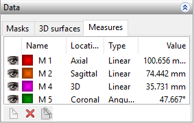
Fig. 164 Data management.#
Simultaneous Viewing of Images and Surfaces#
Images and surfaces can be viewed simultaneously by left-clicking on the shortcut (Fig. 165) located in the lower right corner of the InVesalius interface.

Fig. 165 Shortcut for simultaneous viewing.#
This feature allows users to enable or disable the displaying of images in different orientations (or plans) within the same display window of the 3D surface. Simply check or uncheck the corresponding option in the menu shown in Fig. 166.
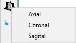
Fig. 166 Selection of the guidelines (plans) to display.#
It is worth noting that when a particular orientation is selected, a check is presented in the corresponding option. This is illustrated in Fig. 167.
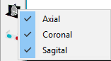
Fig. 167 Selected Guidelines for display.#
If the surface is already displayed, the plans of the guidelines will be presented as shown in Fig. 169. Otherwise, only the plans will be displayed.
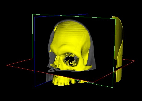
Fig. 168 Surface and plans displayed simultaneously.#
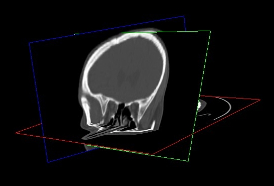
Fig. 169 Flat display (no surface).#
To view the display of a plan, just uncheck the corresponding option in the menu (Fig. 167).
Volume Rendering#
For volume rendering models, InVesalius employs a technique known as raycasting. Raycasting is a technique that simulates the trace of a beam of light toward the object through each screen pixel. The pixel color is based on the color and transparency of each voxel intercepted by the light beam.
InVesalius contains several pre-defined patterns (presets) to display specific tissue types or different types of exam (tomographic contrast, for example).
To access this feature, simply click the shortcut shown in Fig. 170 in the lower right corner of the screen (next to the surface display window) and select one of the available presets.
To turn off volume rendering, click again on the path indicated by Fig. 170 and select the Disable option.

Fig. 170 Shortcut to volume visualization.#
Viewing Standards#
There are several predefined viewing patterns. Some examples are illustrated in the following figures.
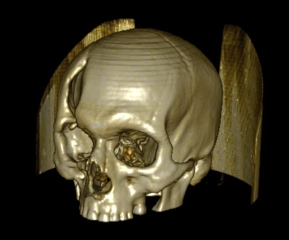
Fig. 171 Bright.#
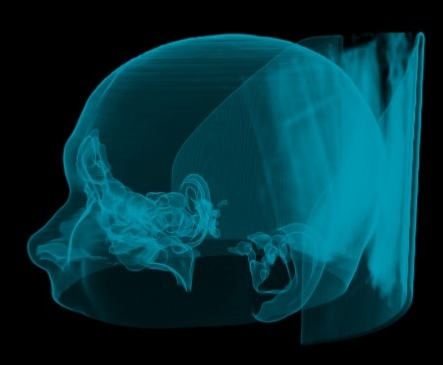
Fig. 172 Airway II.#
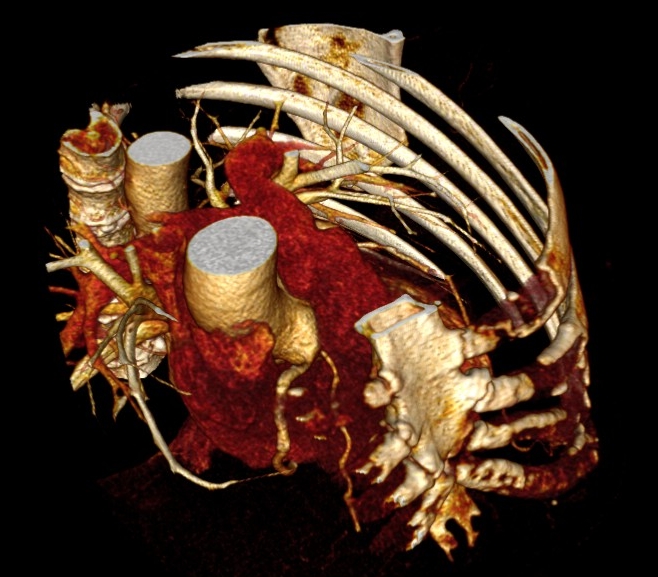
Fig. 173 Contrast Medium.#
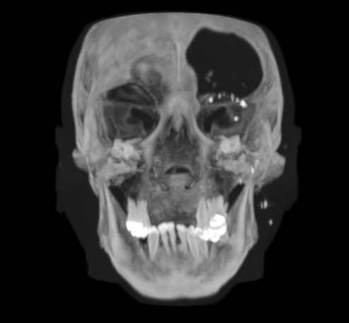
Fig. 174 MIP.#
Standard Customization#
Some patterns can be personalized (and customized). Fig. 175 is exhibiting a pattern and some graphical controls’ adjustment. With these features, the color of a given structure and its opacity can be altered, determining if and how it will be displayed.
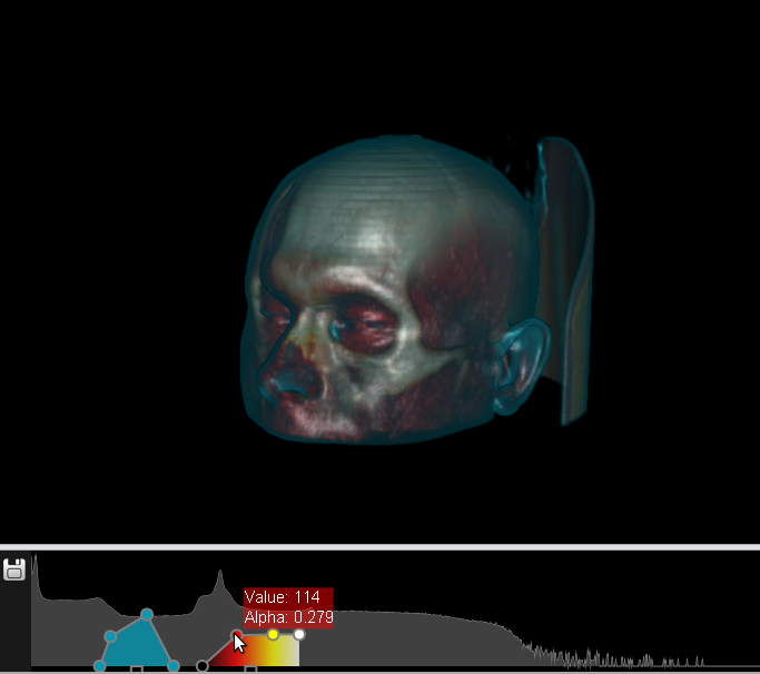
Fig. 175 Settings for the display pattern Soft Skin + II.#
To hide a structure, use the control setting chart to decrease the opacity of the corresponding region. In the example in Fig. 175 suppose we want to hide the muscular part (appearing in red). To do this, simply position the pointer over the muscular part in red and, using the left mouse button, drag the point down to reduce opacity and make the part transparent. Fig. 176 illustrates the result.
Note: The Alpha value indicates the opacity of the color and the value, the color intensity of the pixel.
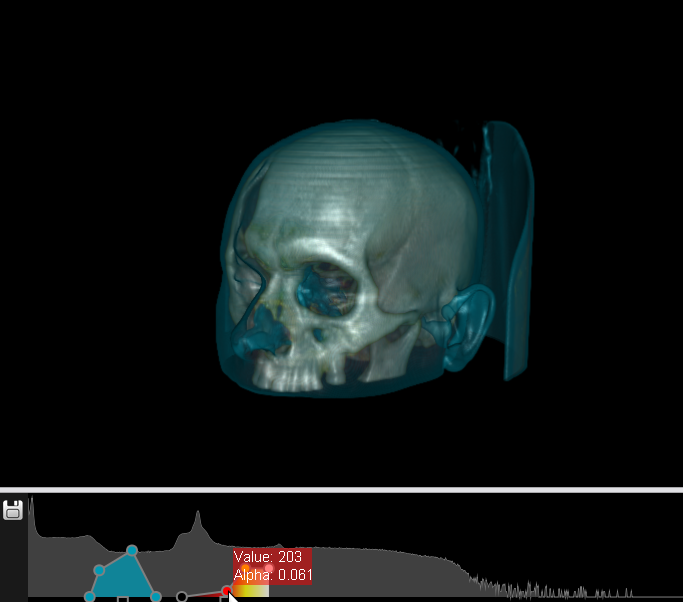
Fig. 176 Display Standard Soft Skin + II changed.#
We can also remove or add points on the graph control setting. To remove, simply click with the right mouse button on the point. To add a new point, click the left button on the line graph. One can also save the resulting pattern by clicking the shortcut shown in Fig. 177.

Fig. 177 Shortcut to save standard.#
To save the pattern, InVesalius displays a window like the one shown in Fig. 178. Enter a name for the custom pattern and click OK. The saved pattern will be available for the next time the software is opened.
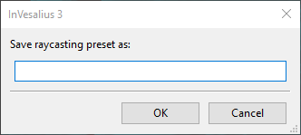
Fig. 178 Window to save name of pattern.#
Standard Customization with Brightness and Contrast#
You can customize a pattern without using the graphical control settings presented in the previous section. This is done through the brightness and contrast controls on the toolbar. Activate these by clicking the icon shown in Fig. 179.
Fig. 179 Shortcut to Brightness and Contrast.#
Enable the control by dragging the mouse, with the left button pressed on the volume window. This will change the values of the window width and window level. The procedure is the same as with slices applied to 2D images, which can be seen in Brightness and contrast. Dragging the mouse in a horizontal direction changes the window level value; drag left to decrease and right to increase. Dragging the mouse vertically changes the value of window width; drag down to decrease and up to increase.
Manipulating these values can be useful for different viewing results. For example, to add tissue to the display, drag the mouse diagonally with left button pressed from the lower right to the upper left corner of the preview window. To remove tissue visualization, do the opposite, (i.e., drag the mouse diagonally from top left to bottom right with the left button pressed). See Fig. 180.
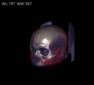
Fig. 180 Raycasting.#
Cut#
In volume rendering, the cut function is used to view a cross-section of a region. With a volume pattern selected, click Tools, and then click Cut plane (Fig. 181).
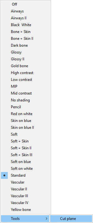
Fig. 181 Enabling plan to cut.#
An outline for cutting appears next to the volume. To make the cut, hold the left mouse button on the plane and drag the mouse. To rotate the plane, hold the left mouse button pressed on its edge and move the mouse in the desired direction as shown in Fig. 182.
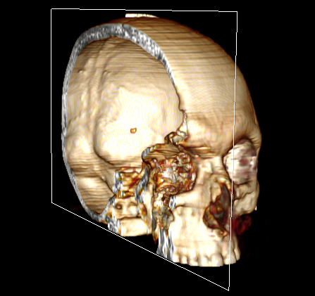
Fig. 182 Image with clipping plane.#
When finished using the function, click Tools and again click Cut plane (Fig. 182).
Stereoscopic Visualization#
InVesalius supports stereoscopic visualization of 3D models. First, a surface (see Surfaces) or an active volumetric visualization (see Volume rendering) must be created. Then, click the icon (shown in Fig. 183) on the bottom right part of the interface and choose the desired projection type (Fig. 184).

Fig. 183 Shortcut to activate stereoscopic viewing methods.#
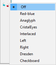
Fig. 184 Different methods of stereoscopic visualization.#
InVesalius supports the following types of stereoscopic viewing:
Red-blue
Anaglyph
CristalEyes
Interlaced
Left
Right
Dresden
Checkboard
Figures below present three different types of projections.
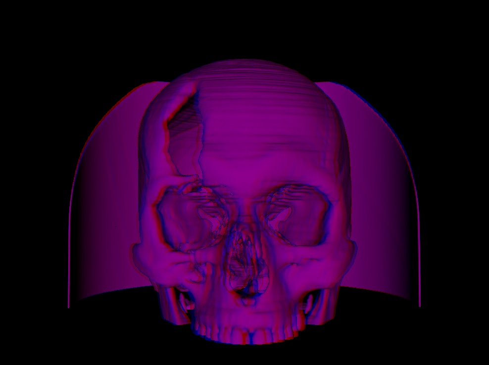
Fig. 185 Red-blue projection.#
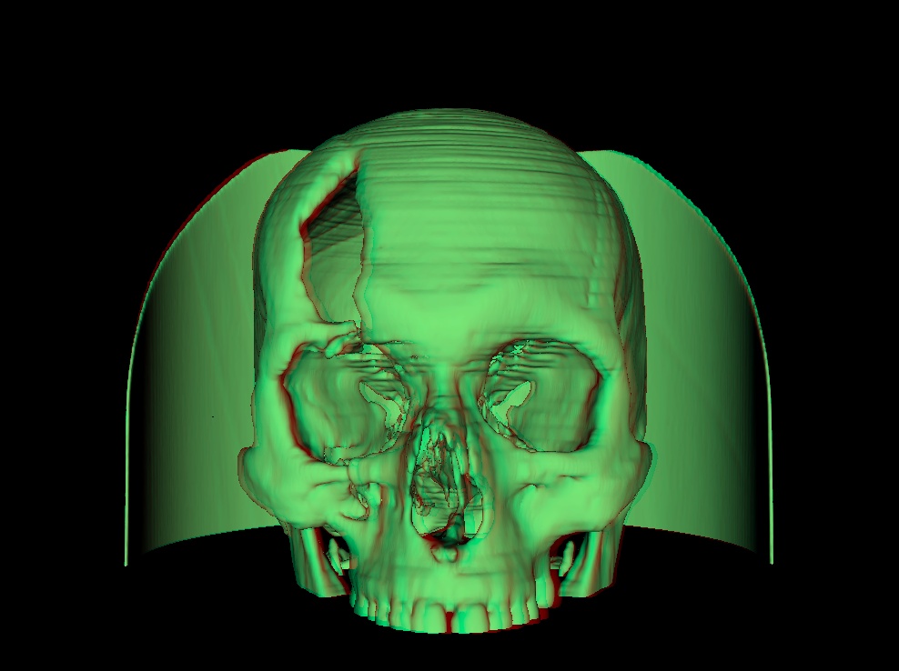
Fig. 186 Anaglyph projection.#
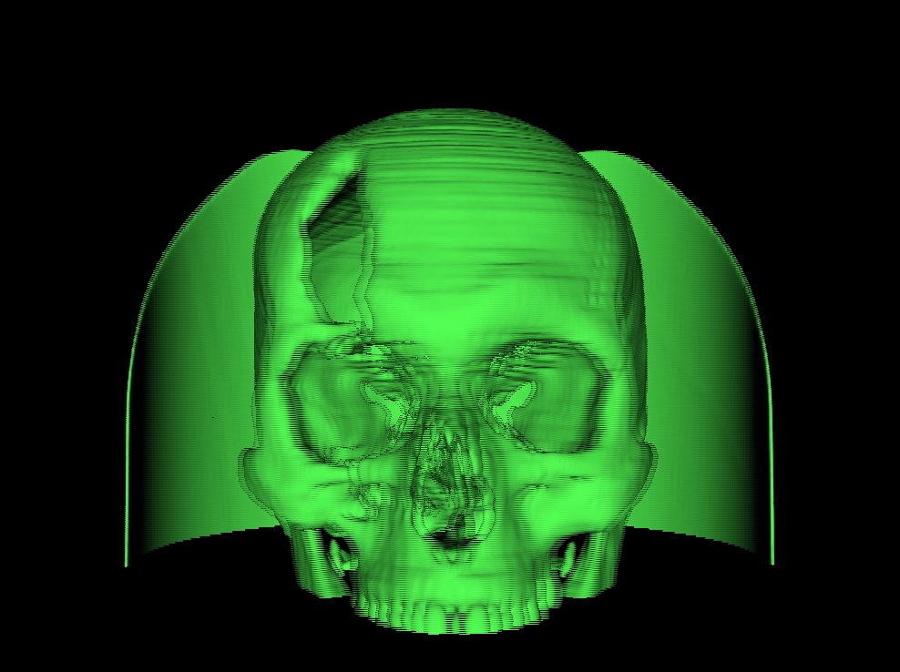
Fig. 187 Interlaced projection.#
Data Export#
InVesalius can export data in different formats, such as OBJ, STL and others, to be used in other software.
The menu to export data is located in the left panel of InVesalius, inside item 4. Export data (displayed below in Fig. 188). If the menu is not visible, double-click with the left mouse button to expand the item.
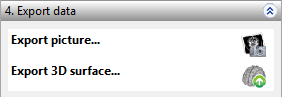
Fig. 188 Menu to export data.#
Surface#
To export a surface, select it from the data menu as shown in Fig. 189.
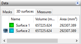
Fig. 189 Select surface to be exported.#
Next, click on the icon shown in Fig. 190.

Fig. 190 Shortcut to export surface.#
When the file window displays (as shown in Fig. 191), type the file name and select the desired exported format. Finally, click Save.
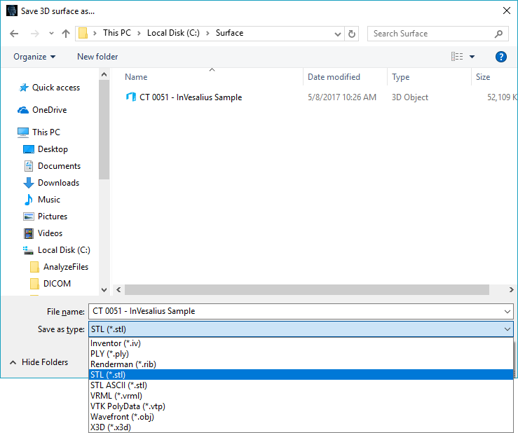
Fig. 191 Window to export surface.#
Files formats available for exportation in InVesalius are listed in the table below.
Format |
Extension |
|---|---|
Inventor |
.iv |
Polygon File Format |
.ply |
Renderman |
.rib |
Stereolithography (binary) |
.stl |
Stereolithography (ASCII) |
.stl |
VRML |
.vrml |
VTK PolyData |
.vtp |
Wavefront |
.obj |
Image#
Images exhibited in any orientation (axial, coronal, sagittal and 3D) can be exported. To do so, left-click on the shortcut shown in Fig. 192 and select the sub-window related to the target image to be exported.
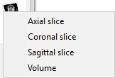
Fig. 192 Menu to export images.#
On the window shown (Fig. 193), select the desired file format, then click Save.
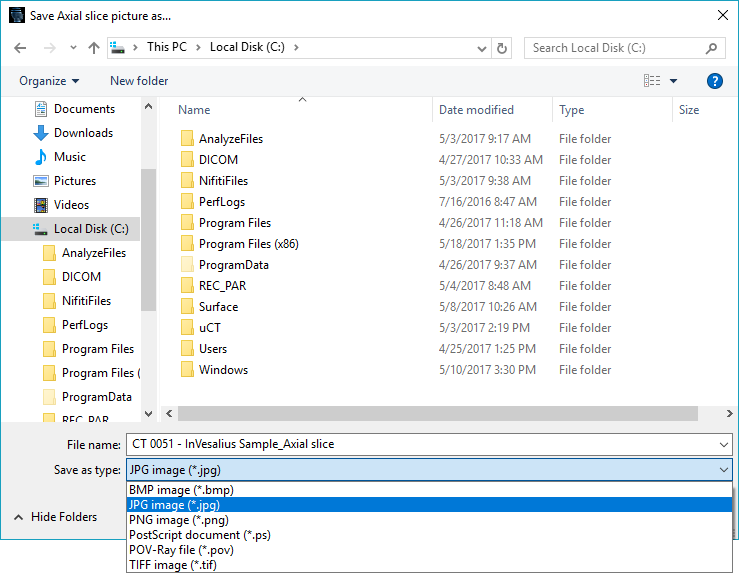
Fig. 193 Window to export images.#
Customization#
Some customization options are available for InVesalius users. They are shown as follows.
Tools Menu#
To hide/show the side tools menu, click the button shown in Fig. 194.

Fig. 194 Shortcut to hide/show side tools menu.#
With the menu hidden, the image visualization area in InVesalius is expanded, as shown in Fig. 195.
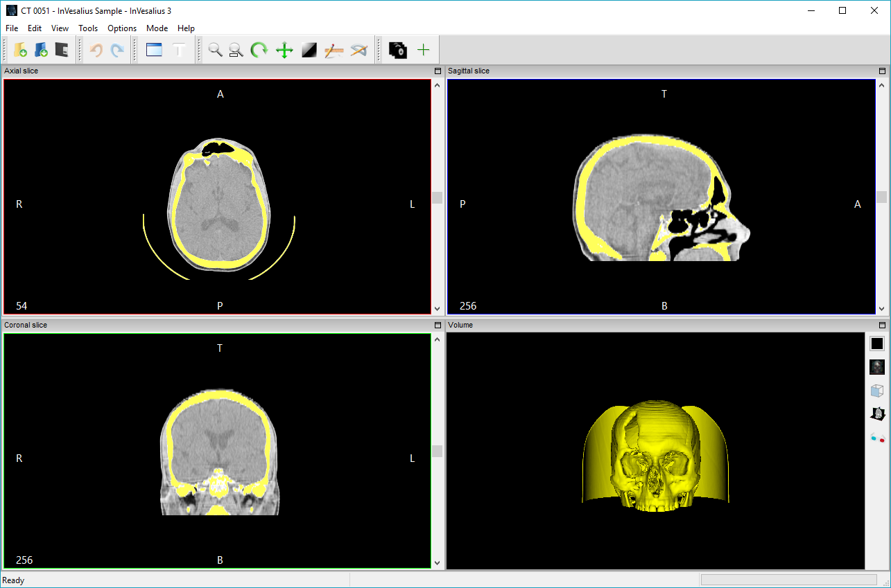
Fig. 195 Side menu hidden.#
Automatic Positioning of Volume/Surface#
To automatically set the visualization position of a volume or surface, click on the icon shown in Fig. 196 (located in the inferior right corner of InVesalius screen) and choose one of the available options for visualization.
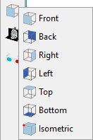
Fig. 196 Options for visualization positioning.#
Background Color of Volume/Surface Window#
To change the background color of the volume/surface window, click on the shortcut shown in Fig. 197. The shortcut is also located in the lower right corner of the InVesalius screen.

Fig. 197 Shortcut to background color of volume/surface window.#
A window for color selection opens (Fig. 198). Next, simply click over the desired color and then click OK.
Fig. 198 Background color selection.#
Fig. 199 illustrates an InVesalius window with the background color changed.
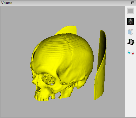
Fig. 199 Background color modified.#
Show/Hide Text in 2D Windows#
To show or hide text in 2D image windows, click on the shortcut illustrated in Fig. 200 on the toolbar.

Fig. 200 Shorcut to show or hide texts.#
Fig. 201 and Fig. 202 show text enabled and disabled, respectively.
Fig. 201 Show texts enabled.#
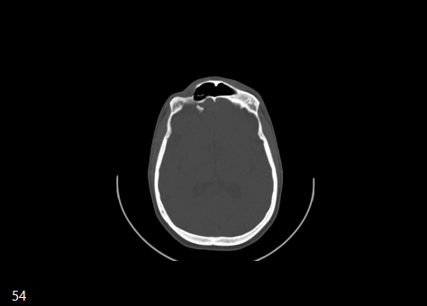
Fig. 202 Show texts disabled.#